An important type of curve maps is based on force-distance data acquired on a regular grid. All major SPM producers offer some regime for the acquisition of such data while the main goal is to map the mechanical properties of the sample. In Gwyddion, these data can be represented as curve maps.
In this section we describe the modules that can be used to handle force-distance curve maps and also give an example of a toolchain for obtaining quantitative nanomechanical results from measured data.
Note that for many of the discussed modules it is important to use curve maps that are already segmented. This means that the approach and retract part of the cuve is marked, either by coming already marked from the instrument, or being marked in Gwyddion using the segmentation module. Also note that the modules assume that the dependent variable is the probe-sample distance - being negative for the indentation part of the curve and positive for the part of the curve when the probe is not touching the surface, as seen on screenshots in this section.
→
The module fits a requested part of the force-distance curve by a polynomial of some and then subtracts it from the whole curve. This is done for every pixel and can be used to remove some unwanted background from the zero line (part of the data where the probe is far from the surface). Parameters and are used to set the dependent and independent variable, which will usually be something probe-sample distance dependent for and something force dependent for . Fitting can be restricted to some particular . The fitting range is entered in percent, so it is recalculated for every pixel based on the curve length, regardless of the absolute offset of the curves.
→
The module fits a requested part of the force-distance curve by a sine function and then subtracts it from the whole curve. This is done for every pixel and can be used to remove some unwanted background related to interference effects from the zero line (part of the data where probe is far from surface). Parameters and are used to set the dependent and independent variable, which will usually be something probe-sample distance dependent for and something force dependent for . Fitting can be restricted to some particular . The fitting range is entered in percent, so it is recalculated for every pixel based on the curve length, regardless of the absolute offset of the curves.
→
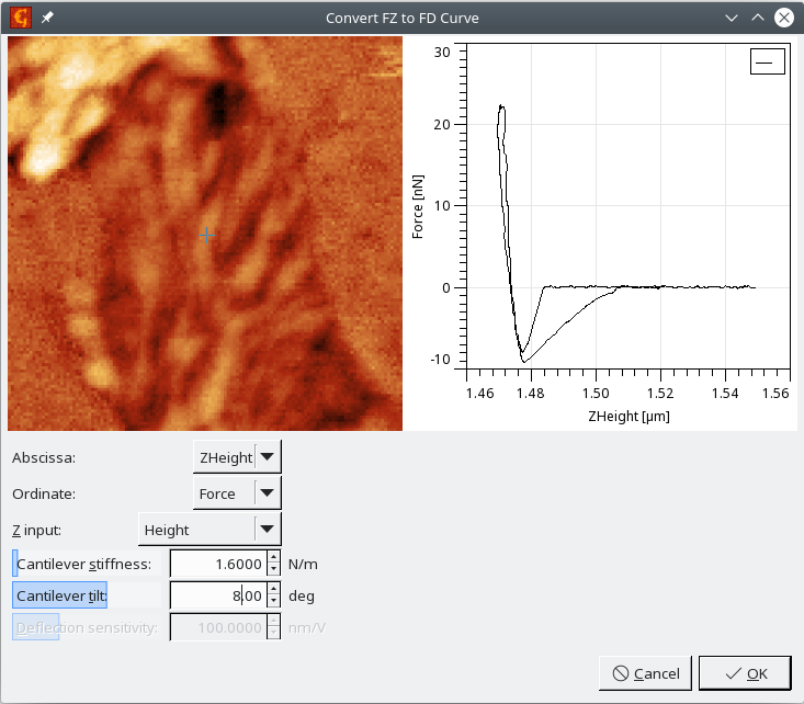
The module performs the conversion of the independent variable in force-distance curves from z-piezo related information (often called z-piezo, height, etc.) to the separation between probe and sample, here called distance. This takes into account the impact of finite cantilever stiffness, which deflects during the force-distance data acquisition. That's why Cantilever stiffness has to be entered. This value can be sometimes found in the metadata, but sometimes might come from another experiment. The lower the cantilever stiffness, the bigger its impact on the curve. A very low value can even change the curve slope to be unrealistic.
Data coming from different instruments can use different orientations of the z axis and the option Z input can be used to reflect it. The goal is to get a curve that has its force maximum at the left side, i.e. the x-axis on the graph is the probe-sample displacement, which is negative when the probe is pressed into the sample.
Effective stiffening of the cantilever related to the angle between cantilever and sample surface can be added using the parameter Cantilever tilt. If the data units for force are Volts, the parameter Deflection sensitivity is automatically activated and can be used to convert the data to force values.
→
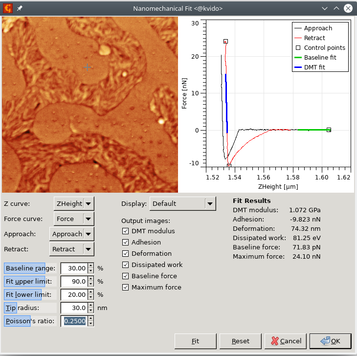
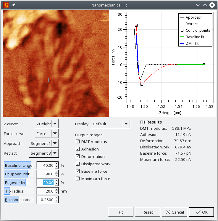
The module performs the automated calculation of simple mechanical properties from force-distance curve maps. The user can enter the ranges in which the baseline (zero line) and the retract part fit will be evaluated and also needs to enter the Tip radius and Poisson's ratio. The right curves need to be picked from the dataset in every pixel and also the right segments need to be selected. These settings are however remembered, so if similar data are processed, there should be no need for setting them.
The adhesion is evaluated as the force between the minimum value on the retract curve and the mean value on the selected part of baseline. Deformation corresponds to the length of the repulsive part of the approach curve, i.e. it is the distance between the position when the force reaches zero after jumping into contact and the position of the maximum force. DMT modulus is determined by fitting a selected part of the retract curve. Dissipation work is calculated as the difference of the integrated approach and retract curves.
The user can select which of these values will be output as arrays and let the module evaluate the data in every pixel using the Fit button.
At the end a set of data fields is produced corresponding to the spatial distribution of different results across the surface.
To illustrate the whole procedure of obtaining nanomechanical results from force-distance curve maps we show here a detailed example how the different modules can be combined.
The data used for this example were produced by Park Systems in the PinPoint regime, using an SD-R30-FM cantilever. The sample is formed by two blended polymers. The input file is available for download. As curve maps are always quite memory demanding, we strongly encourage you to use ithe 64 bit version of the operating system for handling them.
To go step by step and get the same results as provided in the processed file, the following procedure has to be done:
- Right click on the data, open the metadata browser and write down the forceConstant value, which is the cantilever stiffness for this particular experiment.
- Add segments to the data using Cut to Segments module. Use Approach/Retract segmentation mode, and ZHeight curve. Output type should be 'Mark'.
- Use FZ to FD curve module to remove the impact of cantilever stiffness from the data, i.e. to convert the cantilever base height to probe-sample distance. We will use our cantilever stiffness here. Note that it is different from the manufacturer's specifications, so it was probably measured during the experiment, which is an important step towards quantitative measurements. Choose ZHeight for Abscissa, Force for Ordinate and Height as the Z Input.
- Calculate the results using the Nanomechanical Fit module, using the settings shown below: Within the module you can recalculate and preview the individual channels. After clicking on the OK button, you should obtain a set of images representing the spatial distribution of different nanomechanical parameters.