Beside functions for analysis of measured data, Gwyddion provides several generators of artificial surfaces and measurement artefacts that can be used for testing or simulations also outside Gwyddion [1].
All the surface generators share a certain set of parameters, determining the dimensions and scales of the created surface and the random number generator controls. These parameters are described below, the parameters specific to each generator are described in the corresponding subsections.
Image parameters:
- Horizontal, Vertical size
The horizontal and vertical resolution of the generated surface in pixels.
- Square image
This option, when enabled, forces the horizontal and vertical resolution to be identical.
- Width, Height
The horizontal and vertical physical dimensions of the generated surface in selected units. Note square pixels are assumed so, changing one causes the other to be recalculated.
- Dimension, Value units
Units of the lateral dimensions (Width, Height) and of the values (heights). The units chosen here also determine the units of non-dimensionless parameters of the individual generators.
Clicking this button fills all the above parameters according to the current image.
Note that while the units of values are updated, the value scale is defined by generator-specific parameters that might not be directly derivable from the statistical properties of the current image. Hence these parameters are not recalculated.
- Replace the current image
This option has two effects. First, it causes the dimensions and scales to be automatically set to those of the current image. Second, it makes the generated surface replace the current image instead of creating a new image.
- Start from the current image
This option has two effects. First, it causes the dimensions and scales to be automatically set to those of the current image. Second, it makes the generator to start from the surface contained in the current image and modify it instead of starting from a flat surface. Note this does not affect whether the result actually goes to the current image or a new image is created.
Random generator controls:
- Random seed
The random number generator seed. Choosing the same parameters and resolutions and the same random seed leads to the same surface, even on different computers. Different seeds lead to different surfaces with the same overall characteristics given by the generator parameters.
Replaces the seed with a random number.
- Randomize
Enabling this option makes the seed to be chosen randomly every time the generator is run. This permits to conveniently re-run the generator with a new seed simply by pressing Ctrl-F (see keyboard shortcuts).
Update/preview controls:
- Instant updates
If the checkbox is enabled the surface is recalculated whenever an input parameter changes. This option is available in generators which are relatively fast.
- Progressive preview
If the checkbox is enabled the preview shows the evolution of the surface during the simulation. This option is available in slow generators involving iterative physical simulations. Enabling the progressive generally makes the simulation slightly slower as snapshots need to be taken and displayed.

The spectral synthesis module creates randomly rough surfaces by constructing the Fourier transform of the surface according to specified parameters and then performing the inverse Fourier transform to obtain the real surface. The generated surfaces are periodic (i.e. perfectly tilable).
The Fourier image parameters define the shape of the PSDF, i.e. the Fourier coefficient modulus, the phases are chosen randomly. At present, all generated surfaces are isotropic, i.e. the PSDF is radially symmetric.
- RMS
The root mean square value of the heights (or of the differences from the mean plane which, however, always is the z = 0 plane). Button Like Current Image sets the RMS value to that of the current image.
- Minimum, maximum frequency
The minimum and maximum spatial frequency. Increasing the minimum frequency leads to “flattening” of the image, i.e. to removal of large features. Decreasing the maximum frequency limits the sharpness of the features.
- Enable Gaussian multiplier
Enables the multiplication of the Fourier coefficients by a Gaussian function that in the real space corresponds to the convolution with a Gaussian.
- Enable Lorentzian multiplier
Enables the multiplication of the Fourier coefficients by a function proportional to 1/(1 + k2T2)3/4, where T is the autocorrelation length. So, the factor itself is not actually Lorentzian but it corresponds to Lorentzian one-dimensional power spectrum density which in turn corresponds to exponential autocorrelation function (see section Statistical Analysis for the discussion of autocorrelation functions). This factor decreases relatively slowly so the finite resolution plays usually a larger role than in the case of Gaussian.
- Autocorrelation length
The autocorrelation length of the Gaussian or Lorentzian factors (see section Statistical Analysis for the discussion of autocorrelation functions).
- Enable power multiplier
Enables multiplication of Fourier coefficients by factor proportional to 1/kp, where k is the spatial frequency and p is the power. This permits to generate various fractal surfaces.
- Power
The power p.

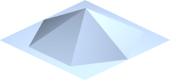
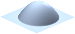
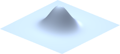
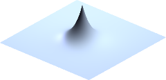
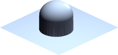
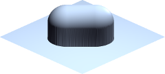
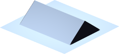
The object placement method permits to create random surfaces composed of features of a specific shape. The algorithm is simple: the given number of objects is placed on random positions at the surface. For each object placed, the new heights are changed to max(z, z0 + h), where z is the current height at a specific pixel, h is the height of the object at this pixel (assuming a zero basis) and z0 is the current minimum height over the basis of the object being placed. The algorithm considers the horizontal plane to be filled with identical copies of the surface, hence, the generated surfaces are also periodic (i.e. perfectly tilable).
|
|
|
|
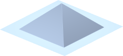
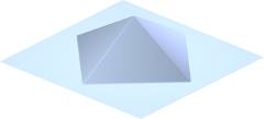
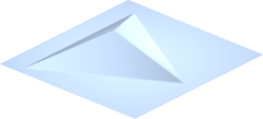
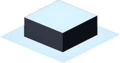
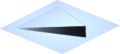
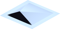
| Pyramid | Diamond | Tetrahedron | Hexagonal pyramid |
|
|
|
|
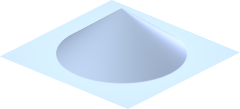
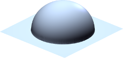
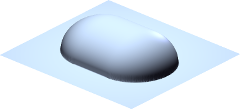
| Cone | Half-sphere | Half-nugget | Parabolic bump |
|
|
|
|
| Gaussian | Exponential spike | Full sphere | Full nugget |
|
|
|
|
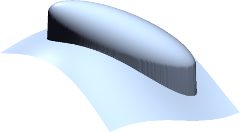
| Box | Thatch | Semi-pyramid | Tent |
| |||
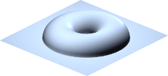
| Doughnut |
Parameters and options in the Shape tab control the shape of individual features:
- Shape
The shape (type) of placed objects. At present the possibilities include half-spheres, boxes, various pyramids, bumps, spikes and a few more weird shapes. The difference between half-sphere and full sphere is in the height. The full sphere includes also the height of the lower half. The same applies to nuggets.
- Size
The lateral object size, usually the side of a containing square.
- Aspect Ratio
The ratio between the x and y dimensions of an object – with respect to some default proportions.
Changing the aspect ratio does not always imply mere geometrical scaling, e.g. objects called nuggets change between half-spheres and rods when the ratio is changed.
- Height
A quantity proportional to the height of the object, normally the height of the highest point.
Enabling Scales with size makes unperturbed heights to scale proportionally to the sizes of individual objects. Otherwise the height is independent on size. Proportional scaling is useful with non-zero size variance to keep the shape of all objects identical (as opposed to elongating and flattening them vertically). If all objects have the same size the option has no effect.
Button Like Current Image sets the height value to a value based on the RMS of the current image.
- Truncate
The shapes can be truncated at a certain height, enabling creation of truncated cones, pyramids, etc. The truncation height is given as a proportion to the total object height. Unity means the shape is not truncated, zero would mean complete removal of the object.
Each parameter can be randomized for individual objects, this is controlled by Variance. For multiplicative quantities (all except orientation and truncation), the distribution is log-normal with the RMS value of the logarithmed quantity given by Variance.
Parameters and options in the Placement tab control where and how the surface is modified using the generated shapes:
- Coverage
The average number of times an object covers a pixel on the image. Coverage value of 1 means the surface would be exactly once covered by the objects assuming that they covered it uniformly and did not overlap. Values larger than 1 mean more layers of objects – and slower image generation.
- Feature sign
The direction in which the surface is changed by adding objects. Positive and negative modifications correspond forming hills and pits adding objects, respectively. Zero value of the parameter means hills and pits are chosen randomly. Positive values mean hills are more likely, while the maximum value 1 means only hills. The same holds for pits and negative values.
- Columnarity
For columnarity of zero the local surface modification works as described in the introduction. For columnarity of one (the maximum), the objects are considered to have also a lower part, which is a perfect mirror of the (visible) upper part. Once the lower object part touches any point on the surface, it sticks to it. This determines the final height. The range of heights grows quckly in this case and the volume is rather porous (not representable with a height field, of course). Values between 0 and 1 mean the object height is interpolated between the two extremes.
- Avoid stacking
When this option is enabled, at most one object may be placed on any pixel of the surface. Hence, they never overlap. The Coverage option then does not determine how many objects are actually placed, but only how many the generator tries. Once there is no free space remaning where an object of given size could be added, increasing the coverage has no effect (beside slowing down the generation).
- Orientation
The rotation of objects with respect to some base orientation, measured anticlockwise. The orientation can be also randomised using the corresponding Variance.

Particle depositions performs a dynamical simulation of interacting spherical particles falling onto a solid surface. The particles do not fall all at once. Instead, they are dropped sequentially among the particles already lying on the surface and left to relax.
- Particle radius
Radius of the spherical particles in real units. The height and lateral dimensions must be the same physical quantity so there is only one dimensional parameter.
- Distribution width
Standard deviation of radius distribution (Gaussian).
- Coverage
How much of the surface would be covered if it was covered uniformly by the deposited particles. If the simulation is unable to place as many particles as requested, usually due to too short time, an error message is displayed.
- Relaxation steps
Simulation length, measured in the number of iterations.
The rod deposition method is based on the same dynamic simulation, but for elongated particles. The particles are in fact formed by sphere triplets, nevertheless this still allows a reasonable range of particle aspect ratios. The simulation also has several more interaction parameters.

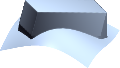
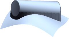
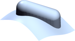
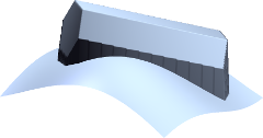
The Objects artificial surface generator is rather fast but at the expense of avoiding any kind of 3D geometry and just moulding the surface using a few simple rules. Particle and rod depositions lie near the other end of the speed-realism spectrum and perform actual dynamical simulation of interacting particles falling onto the surface. This module represents a middle ground, as it forms the surface from real 3D solids, but still using only simple rules for what happens to them when they hit the surface, retaining a good surface generation speed.
The solids start falling in the horizontal position. When they hit the surface, a local mean plane around in the contact area is found. The shape is then rotated to lie flat on this local plane. Its final height is determined as detailed in the description of Columnarity below and then it just sticks in this position. There is no further sliding, toppling or other dynamic settling process.
Several generator parameters have exactly the same meaning as in Objects. This includes Coverage, Avoid stacking and Orientation. The others are explained below:
- Shape
The shape (type) of placed objects. At present the possibilities include various elongated shapes.
- Width
The shapes can be elongated along the x axis (as controlled by Aspect ratio). Their dimension in the orthogonal direction is given by width. The cross section is symmetrical. Therefore, the width determines both the horizontal width and height.
- Aspect ratio
The ratio between the x and y dimensions, in other words, the elongation. It is always at least unity; the shapes are never squashed along the x axis. The aspect ratio distribution can be thus noticeably asymmetrical when the nominal aspect ratio is around unity and the variation is large.
- Columnarity
In general, this parameter influences how much the shapes tend to form columnar structures (porous, if topographical images could represent it). The default value of zero can be imagined as the lower part of the shape melting upon impact and filling the depression it has fallen into. Note that the volume balance is somewhat approximate and the height at which the object settles may be such that sharp spikes on the surface pierce through it.
The maximum columnarity (1) means that once any part of the shape touches the surface, it sticks to it. For smaller positive values the final height is interpolated between the two heights gien by the two approaches.
If columnarity is negative, the shape is rammed into the surface. For the minimum value (−1) it settles at the lowest height for which at least one point of its entire lower boundary would not be below the original surface. Again, for other negative values the final height is interpolated.

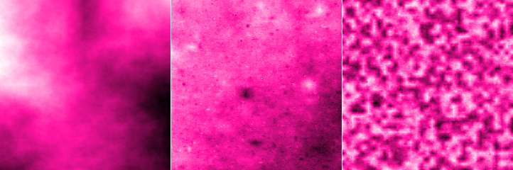
Random uncorrelated point noise is generated independently in each pixel. Several distributions are available.
- Distribution
The distribution of the noise value. The possibilities include Gaussian, exponential, uniform, triangular and salt and pepper distributions.
The salt and pepper distribution works somewhat differently than is usual in computer graphics since the range of values is unbounded. It is a bimodal distribution consiting of two δ-functions. In other words, a constant (given by RMS) is added and/or subtracted from the pixel values.
- Direction
The noise can be generated as symmetrical or one-sided. The mean value of the distribution of a symmetrical noise is zero, i.e. the mean value of data does not change when a symmetrical noise is added. One-sided noise only increases (if positive) or decreases (if negative) the data values.
- RMS
Root mean square value of the noise distribution. More precisely, it is the RMS of the corresponding symmetrical distribution in the case the distribution is one-sided.
- Density
Density is the fraction of values modified. If it is 1 all pixels are modified. When it is smaller some are left intact.

Line noise represents noise with non-negligible duration that leads to typical steps or scars (also called strokes) in the direction of the fast scanning axis – or misaligned scan lines. Parameters Distribution, Direction and RMS have the same meaning as in Point noise. Other parameters control the lateral characteristics of the noise.
The following line defect types are available:
- Steps represent abrupt changes in the value that continue to the end of the scan (or until another step occurs).
- Scars are local changes of the value with a finite duration, i.e. the values return to the original level within the same scan line.
- Ridges are similar to scars but on a larger scale: they can span several scan lines.
- Tilt perturbs the slope of individual scan lines, as opposed to directly shifting heights.
- Hum adds a quasi-periodic disturbance, simulating a type of noise originating from electronic interference.
Steps have the following parameters:
- Density
Average number of defects per scan line, including any dead time (as determined by parameter Within line).
- Within line
Fraction of the time to scan one line that corresponds to actual data acquisition. The rest of time is a dead time. Value 1 means there is no dead time, i.e. all steps occur within the image. Value 0 means the data acquisition time is negligible to the total line scan time, consequently, steps only occur between lines.
- Scanning direction
If steps can occur inside a scan line it determines the horizontal scanning direction (assuming the slow axis scan is from top to bottom). For left to right scanning the left part of the scan line is contiguous with the data above and the right part with data below. For right to left scanning it is the opposite. The two directions are illustrated in the descriptions of Block line correction which corrects similar artefacts.
- Cumulative
For cumulative steps the random step value is always added to the current value offset; for non-cumulative steps the new value offset is directly equal to the random step value.
Scars have the following parameters:
- Coverage
The fraction of the the image covered by defect if they did not overlap. Since the defect may overlap, coverage value of 1 does not mean the image is covered completely.
- Length
Scar length in pixels.
- Variance
Variance of the scar length, see Objects for description of variances.
Ridges have the following parameters:
- Density
Average number of defects per scan line, including any dead time (as determined by parameter Within line).
- Within line
Fraction of the time to scan one line that corresponds to actual data acquisition. The rest of time is a dead time. Value 1 means there is no dead time, i.e. all value changes occur within the image. Value 0 means the data acquisition time is negligible to the total line scan time, consequently, value changes only occur between lines.
- Scanning direction
If steps can occur inside a scan line it determines the horizontal scanning direction (assuming the slow axis scan is from top to bottom). For left to right scanning the left part of the scan line is contiguous with the data above and the right part with data below. For right to left scanning it is the opposite. The two directions are illustrated in the descriptions of Block line correction which corrects similar artefacts.
- Width
Mean duration of the defect, measured in image size. Value 1 means the mean duration will be the entire image scanning time. Small values mean the defects will mostly occupy just one scan line.
Tilt has the following parameters:
- Offset dispersion
With zero offsets all scan lines are tilted around the middle. In other words, the central image column remains unperturbed. Increasing the dispersion of the offsets moves the pivot points randomly more and more to left or right.
Hum has the following parameters:
- Wavelength
Characteristic wavelength of the hum, measured in the image.
- Spread
Small spread means the noise is very narrow-band and looks more or less like as a pure sine wave. Large values produce a wider spectrum with beats and more distorted profile.
- Components
The number of random sine wave components that are used to construct the hum in each scan line.
Different types of line noise added to an artificial pyramidal surface. Top row: unmodified surface (left); relatively sparse cumulative steps (centre); relatively sparse ridges (right). Bottom row: scars of mean length of 16 px and high coverage (left); tilt with small offset dispersion (centre); hum with default settings (right).

Regular geometrical patterns represent surfaces often encountered in microscopy as standards or testing samples. Currently it can generate the following types of pattern:
- Staircase
One-dimensional staircase pattern, formed by steps of constant width and height.
- Grating
One-dimensional pattern, formed by double-sided steps (ridges) constant width and height.
- Amphitheatre
Superellipse-shaped pattern formed by concentric steps of constant width and height.
- Concentric rings
Superellipse-shaped pattern formed by concentric double-sided steps (ridges) of constant width and height.
- Siemens star
Radial pattern formed by alternating high and low wedges.
- Holes (rectangular)
Two-dimensional regular arrangement of rectangular holes, possibly round.
- Pillars
Two-dimensional regular arrangement of symmetrical pillars of several possible shapes (circular, square or hexagonal).
- Double staircase
Two-dimensional regular arrangement of steps of fixed width and height.
Each type of pattern has its own set of geometrical parameters determining the shape and dimensions of various part of the pattern. They are described in the following sections. Most geometrical parametrs have an associated variance control, similar to Object synthesis, which permits making some aspects of the pattern irregular.
The placement of the pattern in the horizontal plane is controlled by parameters in tab Placement, common to all pattern types:
- Orientation
The rotation of the pattern with respect to some base orientation, measured anticlockwise.
This tab also contains the deformation parameters. While enabling the variation of geometrical parameters makes the generated surface somewhat irregular the shape of its features is maintained. Deformation is a complementary method to introduce irregularity, specifically by distorting the pattern in the xy plane. It has two parameters:
- Amplitude
The magnitude of the lateral deformation. It is a relative numerical quantity essentially determining how far the deformation can reach.
- Lateral scale
The characteristic size of the deformations. It describes not how far the features are moved but how sharply or slowly the deformation itself changes within the horizontal plane.
The deformation is analogous to the two-dimensional Gaussian deformation applied by Displacement field. However, it is applied to coordinates before rendering the pattern, whereas Displacement field distorts already sampled images.
All patterns also have a Height parameter, giving the height of features in physical units. For staircase-like patterns that grow continuously it is the height of a single step. For patterns consisting of bumps of holes in a flat base plane it is the height of each individual feature (unless modified by variance).
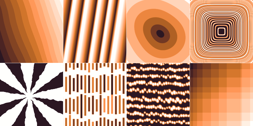
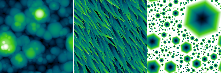
Artificial pattern surfaces. Top row: sharp steps with long-wavelength deformation, scaled grating with large width variance and wide asymmetrical slopes, a slightly deformed amphitheatre with negative parabolicity, and concentric rings with positive parabolicity and varying height. Bottom row: Siemens star with enlarged upper surface, long rectangular holes with varying vertical dimension and position, rows of slightly deformed circular pillars, and double staircase with irregular step width.
Staircase has the following specific parameters:
- Terrace width
The width of one step, given in pixels but also displayed in physical units. All other lateral dimensions are given as fractions of this base width.
The width includes the slope width and can be seen as a “period” of the pattern.
- Position variance
Randomisation of the position of step edge. The edges never cross. Even for the maximum randomness, they can at most move to touch the next edge.
- Slope width
Fraction of width taken by the sloping edge. Zero means sharp edges, one means the pattern will be a flat ramp (without randomness or other modifying parameters).
- Scales with width
If enabled for the step height, the heights will be adjusted to be proportional to the widths of surrounding terraces, while keeping the average step height as given. This more closely preserves the mean plane of the surface even for randomised terrace width.
Grating has the following specific parameters:
- Period
The period of the pattern, given in pixels but also displayed in physical units. All other lateral dimensions are given as fractions of this base width.
- Position variance
Randomisation of the widths of individual ridge-trough pairs.
- Scale features with width
If enabled then all lateral dimensions scale with the width of each individual ridge-trough pair for randomised patterns. Otherwise Top fraction or Slope width refer to the unperturbed base period.
- Top fraction
Fraction of width taken by the upper surface.
- Slope width
Fraction of width taken by the sloping edges. Slopes are added to the top surface; they do not replace it. Therefore, zero Top fraction and non-zero slope results in a triangular profile.
- Asymmetry
Distribution of slope width to left and right edges. Minus one means left edges are sloped and right edges are sharp. Plus one means left edges are sharp and right edges are sloped. Zero means symmetrical slopes.
Amphitheatre has the following specific parameters:
- Superellipse parameter
Step contours are superellipses described by where p is the parameter. Zero corresponds to squares, the maximum value two corresponds to diamonds, and the default value one corresponds to circles.
- Terrace width
The width of one step, given in pixels but also displayed in physical units. All other lateral dimensions are given as fractions of this base width.
The width includes the slope width and can be seen as a “period” of the pattern.
- Position variance
Randomisation of the position of step edge. The edges never cross. Even for the maximum randomness, they can at most move to touch the next edge.
- Parabolicity
Positive values means that the terrace become narrower with increasing distance from centre and the overall profile becomes close to parabolical. Negative values have the opposite effect, with the overall shape becoming a parabola lying on its side.
- Slope width
Fraction of width taken by the sloping edge. Zero means sharp edges, one means the pattern will be become a cone (without randomness or other modifying parameters).
Concentric rings have the following specific parameters:
- Superellipse parameter
Ring contours are superellipses described by where p is the parameter. Zero corresponds to squares, the maximum value two corresponds to diamonds, and the default value one corresponds to circles.
- Period
The period of the pattern, given in pixels but also displayed in physical units. All other lateral dimensions are given as fractions of this base width.
Since the patern is radial, the period must be understood as observed when travelling from the centre outwards.
- Position variance
Randomisation of the widths of individual ridge-trough pairs.
- Parabolicity
Positive values means that the terrace become narrower with increasing distance from centre and the overall profile becomes close to parabolical. Negative values have the opposite effect, with the overall shape becoming a parabola lying on its side.
- Scale features with width
If enabled then all lateral dimensions scale with the width of each individual ridge-trough pair for randomised patterns. Otherwise Top fraction or Slope width refer to the unperturbed base period.
- Top fraction
Fraction of width taken by the upper surface.
- Slope width
Fraction of width taken by the sloping edges. Slopes are added to the top surface; they do not replace it. Therefore, zero Top fraction and non-zero slope results in a triangular profile.
- Asymmetry
Distribution of slope width to left and right edges. Minus one means inner edges are sloped and outer edges are sharp. Plus one means inner edges are sharp and outer edges are sloped. Zero means symmetrical slopes.
Siemens star has the following specific parameters:
- Number of sectors
The number of circular sectors the plane is divided to. Each sector contain an upper and a lower surface, so the number of edges is twice the number of sectors.
- Top fraction
Fraction of angles taken by the upper surface.
- Edge shift
Shift of edges with respect to spokes meeting in the middle. Positive values mean the upper surface is enlarged by the shift, negative values mean the lower surface is enlarged. The shift does not change the asymptotic top fraction (for radius going to infinity), but it modifies the centre of the pattern.
Rectangular holes have the following specific parameters:
- X period and Y period
The horizontal and vertical period of the pattern, given in pixels but also displayed in physical units. All other lateral dimensions are given as fractions of the smaller of these two sizes.
- Position variance
Randomisation of the positions of the hole with respect to the rectangle centre.
- X top fraction and Y top fraction
Fraction of width taken by the upper surface in horizontal and vertical profiles going through the hole centre. Since the dimensions are given as two fractions, the aspect ratio of the hole scales with the corresponding two periods.
The top surface has generally larger area because some profiles do not cross any holes – and it can be further increased by round corners.
- Slope width
Fraction of size (smaller side of the base rectangle) taken by the sloping edges. The slope is the same in both directions.
Slopes are added to the top surface; they do not replace it. Therefore, zero top fraction and non-zero slope can result in triangular profiles.
- Roundness
Radius of rounded corners, given as a fraction of size (smaller side of the base rectangle).
Pillars have the following specific parameters:
- Shape
The shape of the pillar base, which can be circular, square or hexagonal.
- X period and Y period
The horizontal and vertical period of the pattern, given in pixels but also displayed in physical units. All other lateral dimensions are given as fractions of the smaller of these two sizes.
- Position variance
Randomisation of the positions of the pillar with respect to the rectangle centre.
- Size
Pillar width, given as fraction the size (smaller side of the base rectangle). Pillars are symmetrical and their aspect ratio does not scale with the rectangle.
- Slope width
Fraction of size (smaller side of the base rectangle) taken by the sloping edges. The slope is the same in both directions.
Slopes are added to the top surface; they do not replace it. Therefore, zero top fraction and non-zero slope can result in triangular profiles.
- Orientation
Rotation of individual pillars with respect to the rectangular base lattice. For instance square pillars in the base orientation will look similar to the holes pattern (just inverted), whereas rotated by 45 degrees they can form a checkerboard pattern.

The columnar film growth simulation utilises a simple Monte Carlo deposition algorithm in which small particles are incident on the surface from directions generated according to given paramerters, and they stick to the surface around the point where they hit it, increasing the height there locally. The shadowing effect then causes more particles to stick to higher parts of the surface and less particles to the lower parts. This positive local height feedback leads to the formation of columns. The algorithm considers the horizontal plane to be filled with identical copies of the surface, hence, the generated surfaces are also periodic (i.e. perfectly tilable). The surface generator has the following parameters:
- Coverage
The average number of times a particle is generated above each surface pixel.
- Height
Local height increase occurring when the particle sticks to a pixel. Since the horizontal size of the particle is always one pixel the height is measured in pixels. A height of one pixel essentially means cubical particles, as far as growth is concerned. From the point of view of collision detection the particles are considered infinitely small.
- Inclination
Central inclination angle with which the particles are generated (angle of incidence). The value of zero means very small angles of incidence have the highest probability. Large values mean that the particles are more likely to impinge at large angles than at small angles. But for large direction variance, the distribution is still isotropic in the horizontal plane.
- Direction
Central direction in the horizontal plane with which the particles are generated. Large variance means the distribution is isotropic in the horizontal plane; for small variances the growth is anisotopic.
- Relaxation
Method for determination of the pixel the particle will finally stick to. Two options exist at this moment. Weak relaxation, in which only the two pixels just immediately before collision and after collision are considered and the particle sticks to the lower of them. In the case of strong relaxation, a 3×3 neighbourhood is considered in addition. The particle can move to a lower neighbour pixel with a certain probability before sticking permanently.

Vertical ballistic deposition is one of the simplest fundamental film growth models. Particles fall vertically onto randomly chosen sites (pixels). The height in the site is incremented by the particle height. However, if the new height would be smaller than the height in any of the four neigbour sites, the particle is assumed to stick to the neigbour columns. Thus height at the impact site then becomes the maximum of the neigbour heights instead. This is the only mechanism introducing lateral correlations in the resulting roughness.
The simulation has only a few parameters:
- Coverage
The average number of times a particle is generated above each surface pixel.
- Height
Local height increase occurring when the particle falls onto a pixel.

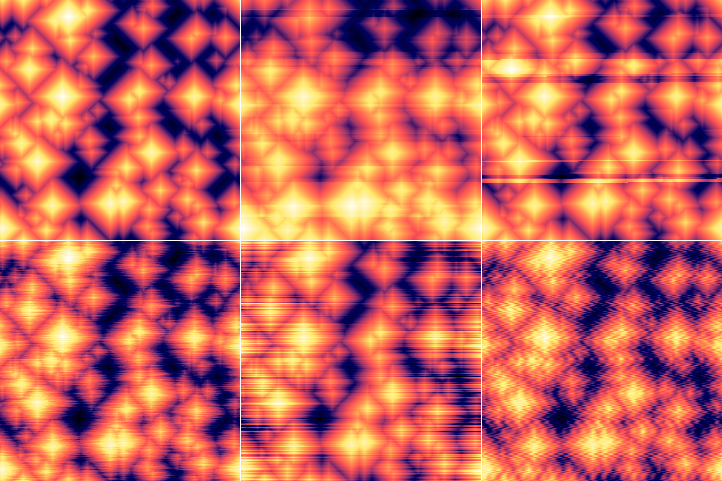
The wave synthesis method composes the image using interference of waves from a number of point sources. Beside the normal cosine wave, a few other wave types are available, each having a cosine and sine form that differ by phase shift π/2 in all frequency components. When the wave is treated as complex, the cosine form is its real part and its sine form is its imaginary part.
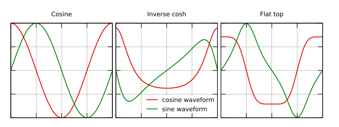
Sine and cosine wave forms for the available wave types. Only the cosine form is used for displacement images; the entire complex wave is used for intensity and phase images.
The generator has the following options:
- Quantity
Quantity to display in the image. Displacement is the sum of the real parts. Amplitude is the absolute value of the complex wave. Phase is the phase angle of the complex wave.
- Number of waves
The number of point sources the waves propagate from.
- Wave form
One of the wave forms described above.
- Amplitude
Approximate amplitude (rms) of heights in the generated image. Note it differs from the amplitude of individual waves: the amplitude of heights in the generated image would grow with the square root of the number of waves in such case, whereas it in fact stays approxiately constant unless the amplitude changes.
- Frequency
Spatial frequency of the waves. It is relative to the image size, i.e. the value of 1.0 means wavelength equal to the lenght of the image side.
- X center, Y center
Locations of the point sources. Zero corresponds to the image centre. The positions are also measured in image sizes. Generally, at least one of the corresponding variances should be non-zero; otherwise all the point sources coincide (some interesting patterns can be still generated with varying frequency though).
- Decay
Decay determines how quickly the waves are attenuated. The value is measured in inverse wavelengths and given as a decimal logarithm, indicated by the units log₁₀.

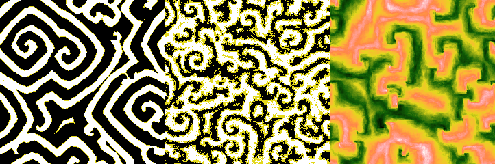
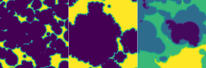
The simulation implements a hybrid non-equilibrium Ising model [2], combining a discrete short-scale discrete Ising model with continuous slow inhibitor.
The discrete variable u has two possible values, between which it can flip probabilistically with probability
where ΔE is the change of energy resulting from flipping and T is the temperature. The energy is given by the number of neighbours in the opposite state in the directions along the coordinate axes no, the number of neighbours in the opposite state in the directions along diagonals nd and also by bias caused by the inhibitor field v:
The continuous inhibitor field v is governed by a local differential equation coupled to the variable u:
where μ is the inhibitor coupling and ν is the bias parameter. The boundary conditions of the simulation are periodic, hence, the generated images are also periodic (i.e. perfectly tilable).
The calculation has the following parameters:
- Number of iterations
One iteration consists of four steps: A Monte Carlo update of u, a time step of solution of the differential equation for v, another Monte Carlo step and another differential euqation time step. The values of v shown correspond to the second update. The quantity shown as u is the average from the two values surrounding in time the corresponding value of v. Hence the images of u are three-valued, not two-valued.
- Temperature T
Temperature determines the probability with which the two-state variable u can flip to the other value if it results in a configurations with higher energy or similar (flips that lower the energy a lot occur unconditonally). A larger temperature means less separation between the two u domains.
- Inhibitor strength B
Strength with which the continuous variable biases the energy of each pixel. For large values the inhibitor has larger influence compared to the surface tension.
- Inhibitor coupling μ
Coupling factor between u and v in the differential equation for v.
- Bias ν
Bias in the differential equation for v towards larger or smaller values.
- Monte Carlo time step
Time step in the differential equation corresponding to one Monte Carlo step. So this parameter determines the relative speed of the two processes.
- Height
Range of values of the created images.
Tab Presets contains a few loadable sets of parameters producing interesting patterns. Select a preset and press to load the parameters to the generator. The random seed is not a part of the preset. So the output images vary with the seed, but they keep the same general character (luck is also involved; some random seeds result in less interesting images than others).

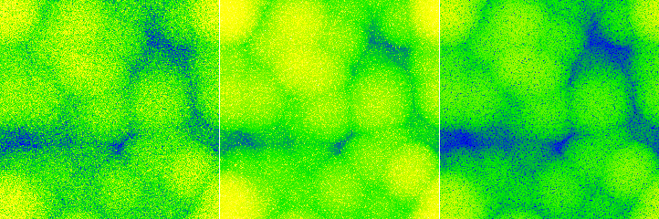
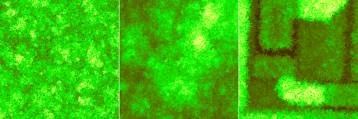
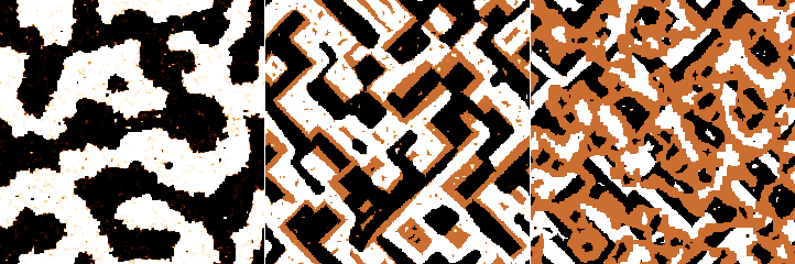
The simulation implements a simple cellular-automaton model of phase separation by annealing an imiscible lattice gas consisting of two components A and C. Only nearest neighbour interaction is considered. The difference of formation energies
determines the preference for phase separation. The annealing proceeds by two neighbour cells (pixels) swaping positions. The always relax to an energentically preferred configuration but they can also switch to energentically less preferred configuration with a probability depending on the temperature T
Since the probability depends only the ratio, we can put the Boltzmann equal to unity and then model depends only on a unitless temperature and relative fractions of the two components.
The calculation has the following parameters:
- Number of iterations
One iteration correspond to each pair of neighbour cell positions being checked for possible swapping once. However, this only holds in probabilistic sense. Some positions can be checked multiple times in one iterations, others not at all.
- Initial temperature
The unitless temperature determines the probability with which cells can swap into less energetically preferred configuration, as described above. The initial temperature is the temperature at which the annealing begins.
- Final temperature
The unitless temperature at which the simulation finishes.
- Component fraction
Fraction of component C in the A–C mixture.
- Height
Range of values of the created images.
- Average iterations
The output image can capture just the final state, or it can be calculated by averaging a certain number of states before the end given by this parameter.
Optionally, a three-component model can be enabled. The third component B behaves identically to A and C. However, the model now has more parameters:
- Fraction of B
The fraction of component B in the mixture. The remainder is divided among A and C according to Component fraction.
- Mixing energy AB
Difference of formation energies for components A and B, relative to the maximum value.
- Mixing energy AC
Difference of formation energies for components A and C, relative to the maximum value.
- Mixing energy BC
Difference of formation energies for components B and C, relative to the maximum value.
In order to keep the unitless temperature scaled consistently with the two-component model, the largest mixing energy is always normalised to 1. If you try to decrease it, the other two mixing energies increase instead, preserving the ratio, until one of them reaches the value 1. Then this energy difference becomes the largest and the previously largest one can be decreased further.

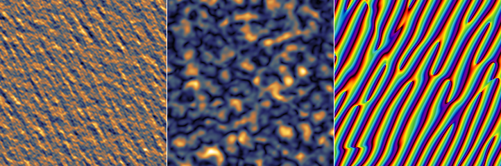
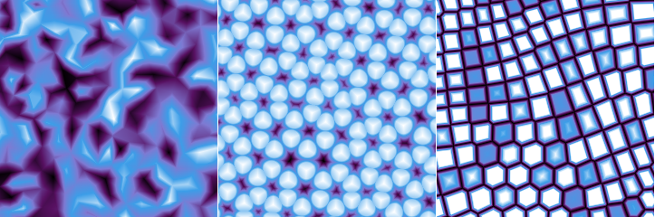
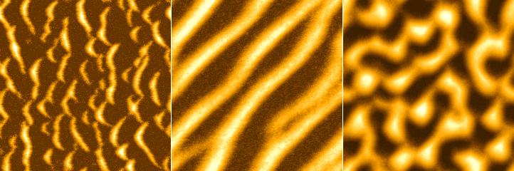
A number of interesting patterns can be generated by solving numerically coupled non-linear partial differential equations in the image plane. At present the module implements two generators with a common basic parameters:
- Number of iterations
The number of time steps when solving the coupled PDEs. Usually the state more or less ceases to evolve after a certain number of iterations – which, however, varies wildly with the pattern type and its parameters.
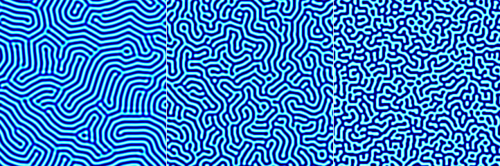
The Turing pattern generator can generate the single classic pattern in a relatively controllable manner. It has the following parameters:
- Size
Characteristic width of stripes in the pattern.
- Degree of chaos
An ad hoc parameter controlling the convergence of the solution. Small values produce orderly patterns. However, the equations can take extremely long time to converge for larger sizes. Large values produce more disturbed patterns, but much more quickly.
The pattern is generated by a two-component diffusion-reaction model simulation, with equations for both components of the form
In the equation for the second component the roles are just swapped (and the constants differ). Function f is defined
Constants p, q and r are not controlled directly. They (and the time step) are calculated from size and degree of chaos according to a calibration formula.
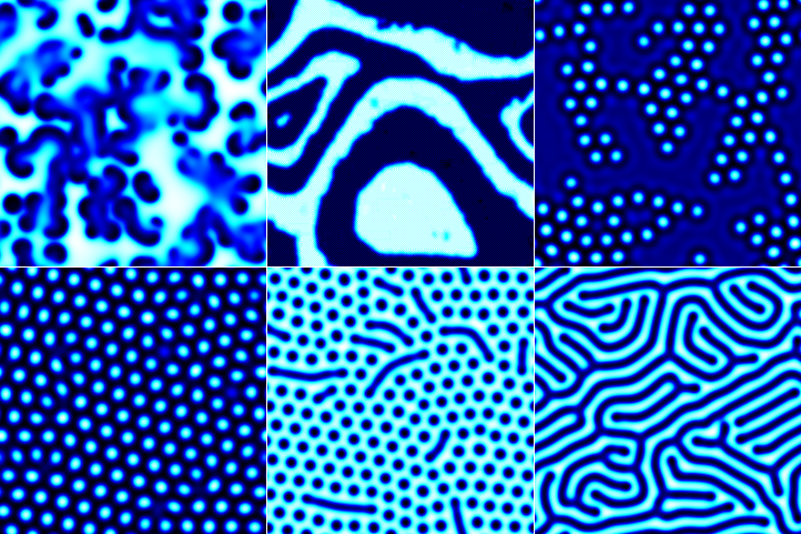
The diffusion reaction model can generate a variety of patterns. However, one adjusts directly the reaction constants and parameters such as feature size are not possible to control. It has the following parameters:
- Output type
Which of the two components should be rendered to the image.
- Removal rate
Removal rate constant for the reaction.
- Feed rate
Feed rate constant for the reaction.
- Source density
The pixel density of fixed sources with low/high values. The density is per pixel, but not the factor 10-3.
- No-source iterations
How many iterations at the end should be carried out with sources removed. It is possible to choose a number larger than the total number of iterations, although it is not very useful (the sources are removed immediately then).
In most parameter ranges the reaction needs a source of reactants to produce interesting patterns. Without such supply the system state evolves to a constant flat image or checkerboard instability. One possibility of forcing an intersting pattern (often used in demonstrations) is a large spatial variation of the reaction constants through the domain. However, this does not allow computation of specific patterns for particular parameter values.
So, instead, the module adds explicit sources. They are realised in a crude manner as random pixels which keep their low/high values (and can be sometimes observed in the animated evolution). They are not subject to the reaction, but they influence their neigbours.
Some patterns are stable once they develop and nothing happens when sources are removed. Some are not and degenerate into one of the non-interesting states. Slightly different sets of patterns can be obtained with sources removed for a long time and with sources removed just briefly at the end. In addition, there are some interesting transitional patterns.

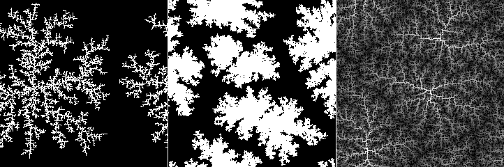
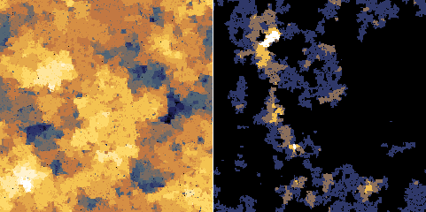
The simulation implements a Monte Carlo discrete diffusion limited aggregation model. Pixel-shaped particles fall onto the surface and move around it until they stick to a cluster, slowly forming a monolayer. The flux of incoming particles is low so that only a few particles are free to move at any given time and the particles can travel a considerable distance on the surface before sticking. For typical parameter values, this leads to the formation of “fractal flake” clusters.
The calculation has the following parameters:
- Coverage
The average number of times a particle falls onto any given pixel. Coverage value of 1 means the surface would be covered by a monolayer, assuming the particles cover it uniformly.
- Flux
The average number particles falling onto any given pixel per simulation step. Smaller values of flux lead to larger structures as the particles diffuse for longer time before they meet another particle. The value is given as a decimal logarithm, indicated by the units log₁₀.
- Height
The height of one particle which gives the height of the steps in the resulting image.
- Sticking probability
The probability that a free particle will finally stick and stop moving when it touches another single particle. Probabilities that the particle will stick if it touches two or three particles increase progressively depending on this value. The sticking probability is always zero for a particle with no neighbours and always one for a particle with all four neighbours.
- Activation probability
The probability a particle that has not stuck will move if it touches another particle. The probability for more touching particles decreases as a power of the single-particle probability. Particles without any neighbours can always move freely.
- Passing Schwoebel probability
A particle that has fallen on the top of an already formed cluster can have reduced probability to descend to the lower layer due to so called Schwoebel barrier. If this parameter is 1 there is no such barrier, i.e. particles can descend freely. Conversely, probability 0 means particles can never descend to the lower layer. The value is given as a decimal logarithm, indicated by the units log₁₀.
Note that some parameter combinations, namely very small flux combined with very small Schwoebel barrier passing probability, can lead to excessively long simulation times.

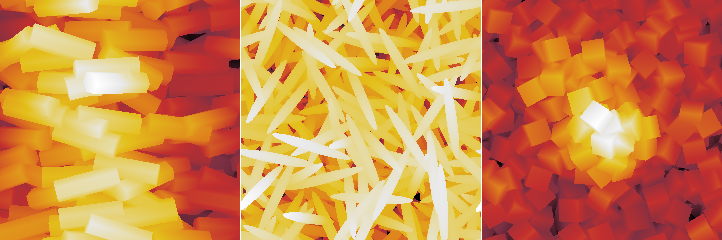
The random fibre placement synthesis method is very similar to Objects, except instead of finite-sized objects it adds infinitely long (in principle) fibres to the surface.
The generator has quite a few parameters, divided into Generator and Placement. The first group contains the basic settings and parameters determining the profiles of individual fibres:
- Shape
The shape of profile across a fibre. Options Semi-circle, Triangle, Rectangle and Parabola are self-explanatory. Quadratic spline shape corresponds to the three-part piecewise quadratic function that is the basis function of quadratic B-spline.
- Coverage
The average number of times a fibre would be placed onto any given pixel. Coverage value of 1 means the surface would be exactly once covered by the fibres assuming that they covered it uniformly and did not overlap. Values larger than 1 mean more layers of fibres – and slower image generation. The value is approximate and the actual coverage depends somewhat on other parameters.
- Width
Fibre width in pixels. It has the usual Variance associated, which determines the difference between entire fibres. However, the width can also vary along a single fibre. This is controlled by the Along fibre option. High values of variation along the fibre can in combination with some other options (in particular high lengthwise deformation and height variation) result in very odd looking images and possibly artefacts.
- Height
A quantity proportional to the height of the fibre, normally the height of the highest point. Similarly to Width, it has two variances, between entire fibres and along each individual fibre.
Enabling Scales with width makes unperturbed heights to scale proportionally with fibre width. Otherwise the height is independent on size.
Button Like Current Image sets the height value to a value based on the RMS of the current image.
- Truncate
The fibres can be truncated at a certain height, enabling creation of profiles in the form of truncated semi-circles, parabolas, etc. The truncation height is given as a proportion to the total fibre height. Unity means the fibre is not truncated, zero would mean complete removal of the fibre.
The second group contains options controlling how fibres are deformed and added to the image:
- Orientation
The rotation of fibres, measured anticlockwise. Zero corresponds to the left-to-right orientation.
- Density
Density controls how frequently the fibre is deformed along its length. Low density means gradual deformation on a large scale, whereas high density means the fibre is deformed often, leading to wavy or curly shapes.
- Lateral
How much the fibre is deformed in the direction perpendicular to its main direction. Increasing this value makes the fibre wavy, but in a relatively regular manner.
- Lengthwise
How much points of the fibre are moved along its length. Increasing this value causes irregular kinks and loops (or even knots) to appear.
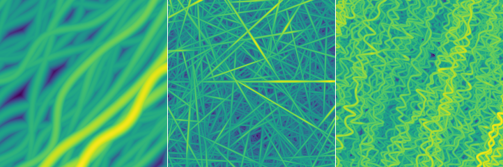

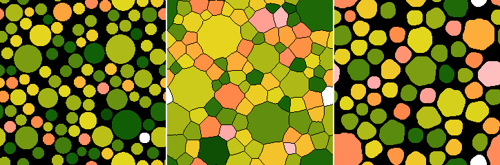
The lattice synthesis module creates surfaces based on randomised two-dimensional lattices. It has two major parts. The first part, controlled by parameters in tab Lattice, is the creation of a set of points in plane that are organised to a more or less randomised lattice. The second part, controlled by parameters in tab Surface, is the actual construction of a surface based on quantities calculated from Voronoi tessellation and/or Delaunay triangulation of the set of points.
The creation of the lattice has the following parameters:
- Lattice
The base lattice type. The random lattice corresponds to completely randomly placed points. Other types correspond to regular organisations of points (square, hexagonal, triangular), well-known tilings (Cairo, snub square, Penrose) or surface reconstructions (silicon 7×7).
- Size
The average cell size. More precisely, this parameter describes the mean point density. It is equal to the side of the square if the same number of points was organised to a square lattice.
- Lattice relaxation
Amount to which the lattice is allowed to relax. The relaxation process pushes points away from very close neighbours and towards large empty space. The net result is that cell sizes become more uniform. Of course, relaxation has no effect on regular lattices. It should be noted that relaxation requires progressive retessellation and large relaxation parameter values can slow down the surface generation considerably.
- Height relaxation
Amount to which the random values assigned to each point (see below) are allowed to relax. The relaxation process is similar to diffusion and leads to overal smoothing of the random values.
- Orientation
The rotation of the lattice with respect to some base orientation, measured anticlockwise. It is only available for regular lattices as the random lattice is isotropic.
- Amplitude, Lateral scale
Parameters that control the lattice deformation. They have the same meaning as in Pattern synthesis.
The final surface is constructed as a weighted sum of a subset of basic quantities derived from the Voronoi tessellation or Delaunay triangulation. Each quantity can be enabled and disabled. When it is selected in the list, its weight in the sum and its thresholding parameters can be modified using the sliders. The lower and upper threshold cut the value range (which is always normalised to [0, 1]) by changing all values larger than the upper threshold equal to the thresold value and similarly for the lower thresold.
Some of the basic quantities are calculated from lateral coordinates only. Some, however, are calculated from random values (“heights”) assigned to each point in the set. The available quantities include:
- Random constant
Rounding interpolation between the random values assigned to each point of the set. This means each Voronoi cell is filled with a constant random value.
- Random linear
Linear interpolation between the random values assigned to each point of the set. Thus the surface is continuous, with each Delaunay triangle corresponding to a facet.
- Random bumpy
An interpolation similar to the previous one, but non-linear, creating relatively level areas around each point of the set.
- Radial distance
Distance to the closest point of the set.
- Segmented distance
Distance to the closest Voronoi cell border, scaled in each cell segment so that the set point is in the same distance from all borders.
- Segmented random
The same quantity as segmented distance, but multiplied by the radndom value assigned to the point of the set.
- Border distance
Distance to the closest Voronoi cell border.
- Border random
The same quantity as border distance, but multiplied by the radndom value assigned to the point of the set.
- Second nearest distance
Distance to the second nearest point of the set.

The module generates, among other things, surfaces with profiles similar to samples of fractional Brownian motion. The construction method is, however, not very sophisticated. Starting from corners of the image, interior points are recursively linearly interpolated along the horizontal and vertical axes, adding noise that scales with distance according to the given Hurst exponent. Some of the surfaces are essentially the same as those generated using spectral synthesis, however, constructing them in the direct space instead of frequency space allows different modifications of their properties.
The generator has the following parameters:
- Hurst exponent
The design Hurst exponent H. For the normal values between 0 and 1, the square root of height-height correlation function grows as H-th power of the distance. The construction algorithm permits formally even negative values beause it stops at the finite resolution of one pixel.
- Stationarity scale
Scale at which stationarity is enforced (note Fractional Brownian motion is not a stationary). When this scale is comparable to the image size or larger, it has little effect. However, when it is small the image becomes “homogeneised” instead of self-similar above this scale.
- Distribution
Distribution of the noise added during the generation. Uniform and Gaussian result in essentially the same surfaces (statistically); the former is faster though. More heavy-tailed distributions, i.e. exponential and especially power, lead to prominent peaks and valleys.
- Power
Power α for the power distribution. The probability density function is proportional to
- RMS
The root mean square value of the heights (or of the differences from the mean plane which, however, always is the z = 0 plane). Note this value applies to the specific generated image, not the process as such, which does not have finite RMS. Button Like Current Image sets the RMS value to that of the current image.

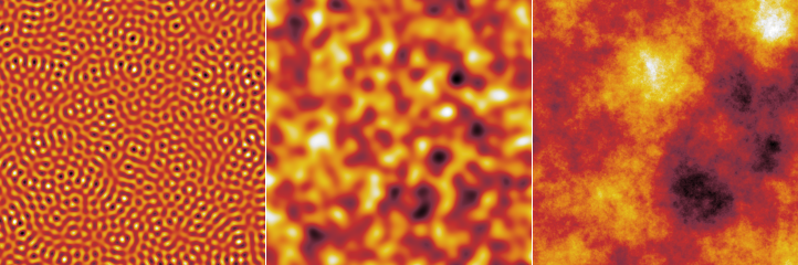
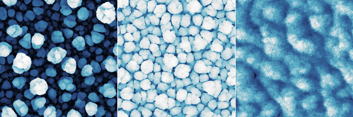
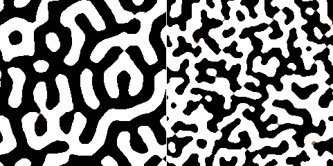
The module creates data somewhat resembling magnetic domain structures that have been studied by magnetic force microscopy (MFM). Unlike more physically correct but very computationally expensive approaches, it works by spectral synthesis of a surface with a limited range of spatial frequencies, and then application of morphological operations to obtain a two-phase image. The output image thus mostly contains of two values representing the two phases, although occasionally a middle “in transition” value can appear.
The generator has the following parameters:
- Size
Typical width of the stripe.
- Size spread
Spread of sizes (or, more precisely, spatial frequencies). Small spread means smooth regular features. However, for very small spread values preferred directions may appear in the image (it becomes anisotropic) due to the exhaustion of allowed spatial frequencies. Large spread means less regular phase boundaries and also more in-transition regions.
- Height
The difference between the values corresponding to the two phases, determining overall z-scale of the image.

The module creates data consisting of non-overlapping discs, possibly post-processed to form a surface covered by tiles. A similar result can be also achieved with Objects when Avoid stacking is enabled. However, in this case the only a few seed discs are placed randomly, the remaining ones are always placed to the middle of the largest remaining empty space. This results in a more uniform distribution of sizes. Furthermore, the transformation to tiles creates structures where typically three tiles meet at angles close to 120 degrees, similarly to foam structures.
The generator has the following parameters:
- Starting radius
Radius of the seed discs placed randomly at the beginnig.
- Minimum radius
The minimum allowed radius of all other discs. When there is no space for a disc of at least this size, the generation stop.
- Separation
Additional separation from neighbour discs. While Minimum radius detemines the minimum size of the actually placed dics, this parameter increases the minimum size of free space allowing placement.
- Transform to tiles
When enabled, all discs are expanded until they would touch their neighbours. The surface becomes tiles, with thin gaps between tiles.
- Gap thickness
Width of gaps between tiles after the tile transformation.
- Apply opening filter
When enabled, the tiling is further post-processed using opening filter of given size. This removes too small tiles and makes the remaning ones rounder.
- Size
Size of the opening filter.
- Height
The height of discs or tiles with respect to the base, determining overall z-scale of the image. Heights of individual features will be spread around this value when Variance is non-zero.

The module is based on a simple simulation of formation of eolian dunes [3]. Particles can be picked up by wind with a certain probability, transferred along the wind direction and deposited in another location. The function has the following parameters:
- Coverage
The average number of particles per one pixel.
- Number of iterations
One iteration correspond to wind picking up randomly one particle in each pixel and deposting it elsewhere. However, the pixels are chosen randomly. Some locations may be chosen multiple times in one iteraton, others not at all. Some selected locations may also be bare bedrock with no sand particle to pick up.
- Direction and Spread
The mean wind direction and wind direction spread. Small spread means the wind direction is consistent. Large values mean more random wind direction.
- Minimum step and Step range
The sand particle can be imagined as only touching the surface occasionally and being carried by the wind high above it between. It can only be deposited when it touches the surface. The minimum step is the minimum distance (in pixels) of one such jump; the range gives the interval (again in pixels) from minimum to maximum jump length.
- Stickng probability on rock
The probability the particle is deposited when it touches the bare bedrock.
- Stickng probability on sand
The probability the particle is deposited when it touches the surface and there is already some sand. This probability should be generally higher than for bare rock.
- Maximum slope
When deposition of a particle (or picking up by wind) creates a too large height difference between neighbour pixels the sand becomes unstable. It then trickles down to either reduce the slopes of a hill for fill holes until the maximum slope is nowhere exceeded.

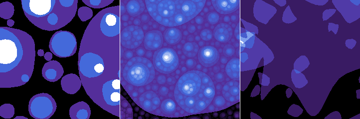
The surface is created by stacking flakes or plateaus on top of each other, starting from the largest and progressing to the smallest according to a scaling law. By default they do not overlap, but it can be enabled to allow overlapping flakes (a bit like those that might occur with 1D materials such as graphene). The generator has the following parameters:
- Maximum size
The approximate maximum radius of a plateau.
- Minimum size
The approximate minimum radius of a plateau.
- Size power law
How fast the plateau size radius decreases with the increasing number of plateaus already there. High values mean the size decreases quickly and plateaus tend to be sparse and isolated. Low values mean the size decreases slowly and plateaus ten to be dense and stacked high.
Warning
It may be difficult, or even impossible, to find positions for all the plateaus with given the maximum and minimum size and scaling power. Low powers are only useful with narrow size ranges. Otherwise the surface generation can be extremely slow – or even never finish at all.- Shape irregularity
How much the shapes can differ from symmetrical discs.
- Overlap fraction
Approximate fraction of plateaus that overlap with another plateau.
- Scale with power of size
The power with which plateau height scales with its radius. For the default power of 0 all pleateaus have the same height (apart from possible random spread). Positive powers mean the height decreases as the size decreased. Negative powers mean smaller plateaus are taller, creating a spiky surface.
The function generates structures resembling resiude of a partially disolved thin film on a flat surface. It is achieved by simple removal of circular regions, either connected or disconnected from already removed parts. It has a the following parameters:
- Coverage
The total area to remove. It is a slight misnomer, because small values mean only a small fraction of the film is dissolved – therefore a lot of the surface is still covered by the residue. It is, nevertheless, consistent with how the term is used in other modules.
- Probability of a new location
The probability that a new independent location is chosen for disolving the film (it may still connect to existing holes by chance). Low values give connected lichen-like holes. Large values give random holes.
- Minimum radius
The minimum radius of circular areas to dissolve.
- Maximum radius
The maximum radius of circular areas to dissolve.
- Size power law
Power with which radius probability decreases. Small values produce mostly only large discs; large values produce mostly only small ones. The default value of 2 corresponds to approximately equal total areas of discs of all sizes.
- Edge width
Width of hole edges in pixesl. Zero leads to a bi-level image. Large values means disolution continues far outside the holes and the outside resembles Euclidean distance to the nearest hole.
Wetting is a simple simulation of wetting front progressing through a random medium. The medium is represented as a voxel grid, where each voxel has a different resistance. The liquid always propagates to the least resistant voxel. The generator produces isotropic patterns with discrete heights corresponding to the levels to which the wetting front have progressed. It has a couple of parameters:
- Coverage
The average number of times the liquid is propagated per pixel. The resulting image shows only the farthest points, so its average value is not in a simple relation to coverage.
- Diffusion
The probability of random propagation from neighbour voxels, not according to the resistance based priority. Note that the value is logarithmic.
[1] D. Nečas, P. Klapetek: Synthetic Data in Quantitative Scanning Probe Microscopy. Nanomaterials 11 (2021) 1746 10.3390/nano11071746
[2] L. M. Pismen, M. I. Monine, G. V. Tchernikov: Patterns and localized structures in a hybrid non-equilibrium Ising model. Physica D 199 (2004) 82, doi:10.1016/j.physd.2004.08.006
[3] B. T. Werner: Eolian dunes: Computer simulations and attractor interpretation. Geology 23 (1995) 1107, doi:10.1130/0091-7613(1995)023<1107:EDCSAA>2.3.CO;2