While analysing randomly rough surfaces we often need a statistical approach to determine some set of representative quantities. Within Gwyddion, there are several ways of doing this. In this section we will explain the various statistical tools and modules offered in Gwyddion, and also present the basic equations which were used to develop the algorithms they utilize.
Scanning probe microscopy data are usually represented as a two-dimensional data field of size N×M, where N and M are the number of rows and columns of the data field, respectively. The real area of the field is denoted as Lx×Ly where Lx and Ly are the dimensions along the respective axes. The sampling interval (distance between two adjacent points within the scan) is denoted Δ. We assume that the sampling interval is the same in both the x and y direction and that the surface height at a given point (x, y) can be described by a random function ξ(x, y) that has given statistical properties.
Note that the AFM data are usually collected as line scans along the x axis that are concatenated together to form the two-dimensional image. Therefore, the scanning speed in the x direction is considerably higher than the scanning speed in the y direction. As a result, the statistical properties of AFM data are usually collected along the x profiles as these are less affected by low frequency noise and thermal drift of the sample.

Statistical quantities include basic properties of the height values distribution, such as variance, skewness and kurtosis. The quantities accessible within Gwyddion by means of the Statistical Quantities tool are divided into several groups.
Moment based quantities are expressed using integrals of the height distribution function with some powers of height. They include the familiar quantities:
- Mean value.
- Mean square roughness or RMS of height irregularities Sq: this quantity is computed from 2nd central moment of data values.
- Grain-wise RMS value which differs from the ordinary RMS only if masking is used. The mean value is then determined for each grain (contiguous part of mask or inverted mask, depending on masking type) separately and the variance is then calculated from these per-grain mean values.
- Mean roughness or Sa value of height irregularities.
- Height distribution skewness computed from 3rd central moment of data values.
- Height distribution kurtosis computed from 4th central moment of data values.
More precisely, RMS (σ), skewness (γ1), and kurtosis (γ2) are computed from central moments of i-th order μi
where z̄ denotes the mean value. The are expressed by the following formulas:
Note that Gwyddion computes the excess kurtosis, which is zero for Gaussian data distribution. Add 3 to obtain the area texture parameter Sku.
Mean roughness Sa is similar to RMS value, the difference being that it is calculated from the sum of absolute values of data differences from the mean, instead of their squares.
It should be noted that quantities such as σ calculated using the standard definitions are biased, especially if any scan line levelling has been done. The Correlation Length tool can calculate bias-corrected quantities. See its description for more details.
Order based quantities represent values corresponding to specific ranks if all the values were ordered. They include:
- The minimum and maximum value and median.
- Maximum peak height Sp, which differs from the maximum by being calculated with respect to the mean height.
- Maximum pit depth Sv, which differs from the minimum by being calculated with respect to the mean height.
- Maximum height Sz, the total value range. It is the difference between minimum and maximum or, equivalently, Sv and Sp.
Hybrid quantities combine heights and spatial relations in the surface and include:
- Projected surface area and surface area: computed by simple triangulation.
- Volume, calculated as the integral of the surface height over the covered area.
- Mean inclination of facets in area: computed by averaging normalized facet direction vectors.
- Variation, which is calculated as the integral of the absolute value of the local gradient.
- Surface slope, which is the mean square local gradient. In other words, the mean square of the local gradient is first calculated. The slope is then obtained as its square root.
The surface area is estimated by the following method. Let zi for i = 1, 2, 3, 4 denote values in four neighbour points (pixel centres), and hx and hy pixel dimensions along corresponding axes. If an additional point is placed in the centre of the rectangle which corresponds to the common corner of the four pixels (using the mean value of the pixels), four triangles are formed and the surface area can be approximated by summing their areas. This leads to the following formulas for the area of one triangle (top) and the surface area of one pixel (bottom):
The method is now well-defined for inner pixels of the region. Each value participates on eight triangles, two with each of the four neighbour values. Half of each of these triangles lies in one pixel, the other half in the other pixel. By counting in the area that lies inside each pixel, the total area is defined also for grains and masked areas. It remains to define it for boundary pixels of the whole data field. We do this by virtually extending the data field with a copy of the border row of pixels on each side for the purpose of surface area calculation, thus making all pixels of interest inner.
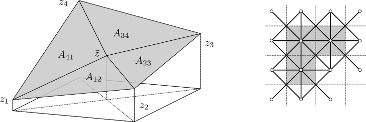
Surface area calculation triangulation scheme (left). Application of the triangulation scheme to a three-pixel masked area (right), e.g. a grain. The small circles represent pixel-centre vertices zi, thin dashed lines stand for pixel boundaries while thick lines symbolize the triangulation. The surface area estimate equals to the area covered by the mask (grey) in this scheme.
In addition, the tool calculates a few quantities that do not belong in any of the previous categories:
- Scan line discrepancy, characterising the differences between scan lines. It can be visualised as follows: if each line in the image was replaced by the average of the two neighbour lines, the new image would differ slightly from the original. Taking the mean square difference and dividing it by the mean square value of the image, we obtain the displayed discrepancy value.
Tip
By default, the Statistical Quantities tool will display figures based on the entire image. If you would like to analyse a certain region within the image, simply click and drag a rectangle around it. The tool window will update with new numbers based on this new region. If you want you see the statistical quantities for the entire image again, just click once within the data window and the tool will reset.
One-dimensional statistical functions can be accessed by using the Statistical Functions tool. Within the tool window, you can select which function to evaluate using the selection box on the left labelled Output Type. The graph preview will update automatically. You can select in which direction to evaluate (horizontal or vertical), but as stated above, we recommend using the fast scanning axis direction. You can also select which interpolation method to use. When you are finished, click to close the tool window and output a new graph window containing the statistical data.
Tip
Similar to the Statistical Quantities tool, this tool evaluates for the entire image by default, but you can select a sub-region to analyse if you wish.The simplest statistical functions are the height and slope distribution functions. These can be computed as non-cumulative (i.e. densities) or cumulative. These functions are computed as normalized histograms of the height or slope (obtained as derivatives in the selected direction – horizontal or vertical) values. In other words, the quantity on the abscissa in “angle distribution” is the tangent of the angle, not the angle itself.
The normalization of the densities ρ(p) (where p is the corresponding quantity, height or slope) is such that
Evidently, the scale of the values is then independent on the number of data points and the number of histogram buckets. The cumulative distributions are integrals of the densities and they have values from interval [0, 1].
The height and slope distribution quantities belong to the first-order statistical quantities, describing only the statistical properties of the individual points. However, for the complete description of the surface properties it is necessary to study higher order functions. Usually, second-order statistical quantities observing mutual relationship of two points on the surface are employed. These functions are namely the autocorrelation function, the height-height correlation function, and the power spectral density function. A description of each of these follows:
The autocorrelation function is given by
where z1 and z2 are the values of heights at points (x1, y1), (x2, y2); furthermore, τx = x1 − x2 and τy = y1 − y2. The function w(z1, z2, τx, τy) denotes the two-dimensional probability density of the random function ξ(x, y) corresponding to points (x1, y1), (x2, y2), and the distance between these points τ.
From the discrete AFM data one can evaluate this function as
where m = τx/Δx, n = τy/Δy. The function can thus be evaluated in a discrete set of values of τx and τy separated by the sampling intervals Δx and Δy, respectively.
For AFM measurements, we usually evaluate the one-dimensional autocorrelation function based only on profiles along the fast scanning axis. It can therefore be evaluated from the discrete AFM data values as
It should be noted that this estimate is biased, especially if any scan line levelling has been done. The Correlation Length too can calculate a bias-corrected ACF. See its description for more details.
The one-dimensional autocorrelation function is often assumed to have the form of a Gaussian, i.e. it can be given by the following relation
where σ denotes the root mean square deviation of the heights and T denotes the autocorrelation length.
For the exponential autocorrelation function we have the following relation
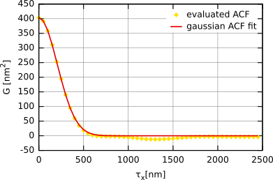
Autocorrelation function obtained for simulated Gaussian randomly rough surface (i.e. with a Gaussian autocorrelation function) with σ ≈ 20 nm and T ≈ 300 nm.
We can also introduce the radial ACF Gr(τ), i.e. angularly averaged two-dimensional ACF, which of course contains the same information as the one-dimensional ACF for isotropic surfaces:
Note
For optical measurements (e.g. spectroscopic reflectometry, ellipsometry) the Gaussian autocorrelation function is usually expected to be in good agreement with the surface properties. However, some articles related with surface growth and oxidation usually assume that the exponential form is closer to the reality.The interface distribution function (IDF) is the second derivative of ACF
Positions and signs of its extrema are linked to features like grains sizes and intergrain distances.
The difference between the height-height correlation function and the autocorrelation function is very small. As with the autocorrelation function, we sum the multiplication of two different values. For the autocorrelation function, these values represented the different distances between points. For the height-height correlation function, we instead use the power of difference between the points.
For AFM measurements, we usually evaluate the one-dimensional height-height correlation function based only on profiles along the fast scanning axis. It can therefore be evaluated from the discrete AFM data values as
where m = τx/Δx. The function thus can be evaluated in a discrete set of values of τx separated by the sampling interval Δx.
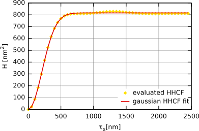
The one-dimensional height-height correlation function is often assumed to be Gaussian, i.e. given by the following relation
where σ denotes the root mean square deviation of the heights and T denotes the autocorrelation length.
For the exponential height-height correlation function we have the following relation
In the following figure the height-height correlation function obtained for a simulated Gaussian surface is plotted. It is fitted using the formula shown above. The resulting values of σ and T obtained by fitting the HHCF are practically the same as for the ACF.
The two-dimensional power spectral density function can be written in terms of the Fourier transform of the autocorrelation function
Similarly to the autocorrelation function, we also usually evaluate the one-dimensional power spectral density function which is given by the equation
This function can be evaluated by means of the Fast Fourier Transform as follows:
where Pj(Kx) is the Fourier coefficient of the j-th row, i.e.
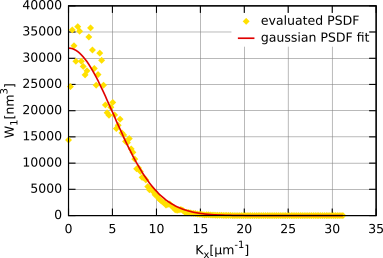
If we choose the Gaussian ACF, the corresponding Gaussian relation for the PSDF is
For the surface with exponential ACF we have
In the following figure the resulting PSDF and its fit for the same surface as used in the ACF and HHCF fitting are plotted. We can see that the function can be again fitted by Gaussian PSDF. The resulting values of σ and T were practically same as those from the HHCF and ACF fit.
We can also introduce the radial PSDF Wr(K), i.e. angularly integrated two-dimensional PSDF, which of course contains the same information as the one-dimensional PSDF for isotropic rough surfaces:
For a surface with Gaussian ACF this function is expressed as
while for exponential-ACF surface as
Tip
Within Gwyddion you can fit all statistical functions presented here by their Gaussian and exponential forms. To do this, fist click within the Statistical Functions tool window. This will create a new graph window. With this new window selected, click on → .The spectral density can also be integrated radially, giving the angular spectrum. Its peaks can be used to identify the image texture direction.
The Minkowski functionals are used to describe global geometric characteristics of structures. Two-dimensional discrete variants of volume V, surface S and connectivity (Euler-Poincaré Characteristic) χ are calculated according to the following formulas:
Here N denotes the total number of pixels, Nwhite denotes the number of “white” pixels, that is pixels above the threshold. Pixels below the threshold are referred to as “black”. Symbol Nbound denotes the number of white-black pixel boundaries. Finally, Cwhite and Cblack denote the number of continuous sets of white and black pixels respectively.
For an image with continuous set of values the functionals are parametrized by the height threshold value ϑ that divides white pixels from black, that is they can be viewed as functions of this parameter. And these functions V(ϑ), S(ϑ) and χ(ϑ) are plotted.
The range distribution is a plot of the growth of value range depending on the lateral distance. It is always a non-decreasing function.
For each pixel in the image and each lateral distance, it is possible to calculate the minimum and maximum from values that do not lie father than the given lateral distance from the given pixel. The local range is the difference between the maximum and minimum (and in two dimensions can be visualised using the Rank presentation function). Averaging the local ranges for all image pixels gives the range curve.
The area scale graph shows the ratio of developed surface area and projected area minus one, as the function of scale at which the surface area is measured. Because of the subtraction of unity, which would be the ratio for a completely flat surface, the quantity is called “excess” area.
Similar to the correlation functions, the area excess can be in principle defined as a directional quantity. However, the function displayed in the tool assumes an isotropic surface – the horizontal or vertical orientation that can be chosen there only determines the primary direction used in its calculation.
Most of the statistical functions support masking. In other words, they can be calculated for arbitrarily shaped image regions. For some of them, such as the height or angle distribution, no further explanation is needed: only image pixels covered (or not covered) by the mask are included in the computation. However, the meaning of the function is less clear for correlation functions and spectral densities.
We will illustrate it for the ACF (the simplest case). The full description can be found in the literature [1]. The discrete ACF formula can be rewritten
where Ωm is the set of image pixels inside the image region for which the pixel m columns to the right also lies inside the region. If we calculate the ACF for a rectangular region, for example the entire image, nothing changes. However, this formula expresses the function meaningfully for regions of any shape. The only missing part is how to perform the computation efficiently.
For this we define ck,l as the mask of valid pixels, i.e. it is equal to 1 for pixels we want to include and 0 for pixels we want to exclude. It then follows that
Furthermore, if image data are premultiplied by ck,l the ACF sum over the irregular region can be replaced by the usual ACF sum over the entire image. Both are efficiently computed using FFT.
It is important to note that the amount of information available in the data about the ACF for given m depends on Ωm. Unlike for entire rectangular images, it does not have to decrease monotonically with increasing m and can vary almost arbitrarily. There can even be holes, i.e. horizontal distances m for which the region contains no pair of pixels exactly this apart. If this occurs Gwyddion replaces the missing values using linear interpolation.
The height-height correlation function is calculated in a similar manner, only the sums have to be split into parts which can be then evaluated using FFT. For PSDF, this is not possible because each Fourier coefficient depends on each data value. So, instead, the cyclic autocorrelation function is calculated in the same manner as ACF, and PSDF is then obtained as its Fourier transform.

The Row/Column Statistics tool calculates numeric characteristics of each row or column and plots them as a function of its position. This makes it kind of complementary to Statistical Functions tool. Available quantities include:
- Mean value, minimum, maximum and median.
- RMS value of the height irregularities computed from data variance Rq.
- Skewness and kurtosis of the height distribution.
- Surface line length. It is estimated as the total length of the straight segments joining data values in the row (column).
- Overall slope, i.e. the tangent of the mean line fitted through the row (column).
- Tangent of β0. This is a characteristics of the steepness of local slopes, closely related to the behaviour of autocorrelation and height-height correlation functions at zero. For discrete values it is calculated as follows:
- Standard roughness parameters Ra, Rz, Rt.
In addition to the graph displaying the values for individual rows/columns, the mean value and standard deviation of the selected quantity is calculated from the set of individual row/column values. It must be emphasised that the standard deviation of the selected quantity represents the dispersion of values for individual rows/columns and cannot be interpreted as an error of the analogous two-dimensional quantity.

The Correlation Length tool can be used for a one-step estimation of image autocorrelation length T from scan lines. The autocorrelation length is estimated using several common methods using either the 1D autocorrelation or 1D power spectral density function. Both functions are plotted on the right side of the dialogue togther with additional information such as their fits by models.
On the left side one can choose the evaluation parameters (beside the common Masking and Orientation options):
- ACF model
- Autocorrelation function type assumed for fitting ACF and PSDF with analytcal models. The model is selected for ACF and the tool uses matching PSDF model automatically.
- Line levelling
- The tool can performs scan line levelling during the estimation (in the selected evaluation direction, which is usually horizontal). It is possible to not apply any levelling by selecting None if lines have already been levelled for instance using Align Rows. However, the bias-corrected evaluation needs to know how they were levelled. You must select degree at least as high as any prior line levelling. Otherwise the results are not valid.
The results of all evaluations are displayed in the middle column, allowing the user to choose the most appropriate one (and compare immediately how much they differ). Note, however, that the `raw' results are biased [2,3] and mainly for comparison and in general should not be used. For ACF-based evaluation, the bias-corrected values [4] are preferred.
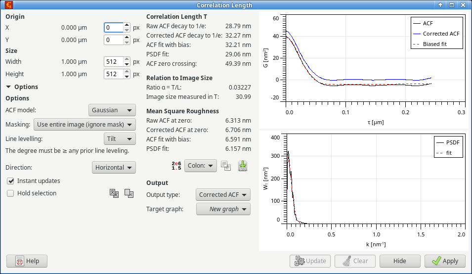
Reported values are split into several section. The correlation length related are defined:
- Raw ACF decay to 1/e
- The horizontal distance at which the discrete ACF (curve ACF) decays to 1/e of its maximum value, which it attains at zero. This is the common definition, matching also the expressions for Gaussian and exponential ACF.
- Corrected ACF decay to 1/e
- The distance at which the bias-corrected ACF (curve Corrected ACF) decays to 1/e of its maximum value.
- ACF fit with bias
- Correlation length obtained from fitting the raw ACF with the selected model. A modified model is used which takes into account that the discrete ACF data are biased [4]. The fit is shown as curve Biased fit. Note that biased should be read as bias-corrected in this context.
- PSDF fit
- Autocorrelation length obtained by fitting the estimated PSDF using the selected model. The model is not modified in any manner, even though a few initial PSDF data points (the most affected by levelling) are excluded.
- ACF zero crossing
- The horizontal distance at which the raw ACF decays to zero. An uncommon, but sometimes useful characteristics of the ACF decay. The zero crossing is also used in the bias-corrected evaluation.
Image size related quantities compare autocorrelation length T and image size L (more precisely scan line length):
- Ratio α = T/L
- This ratio is used for the estimation of bias of roughness parameters due to finite measurement area. The autocorrelation length is taken from the extrapolated decay.
- Image size measured in T
- The inverse of α measures how many autocorrelation lengths fit into one scan line. It carries the same information, but can be easier to imagine.
A crude estimate of the bias can be obtained as follows. It is mainly useful for getting an idea whether the scan size is sufficient, or how much the result may biased – attempting to use it for correction can easily make things worse.
- Estimate α – for instance by this tool.
- Multiply it by the degree of polynomial used for scan line levelling plus one. This means 1 for subtraction of mean value, 2 for tilt correction, 3 for bow correction, etc.
- The result estimates relative bias of measued roughness. The bias is always negative so add minus if it matters.
A similar procedure can be used for 2D background subtraction. However, almost always some row levelling is applied – at least implicitly the subtraction of mean value. And it is then also the dominant source of bias.
Finally, mean square roughness values are also reported:
- Raw ACF at zero
- Mean square roughness calculated from the raw ACF using the relation It corresponds to the standard definition.
- Corrected ACF at zero
- Mean square roughness calculated using the same relation, but from the corrected ACF.
- ACF fit with bias
- Mean square roughness obtained from fitting the raw ACF with the selected model. A modified model is used which takes into account that the discrete ACF data are biased. The fit is shown as curve Biased fit. Note that biased should be read as bias-corrected in this context.
- PSDF fit
- Mean square roughness obtained by fitting the estimated PSDF using the selected model. The model is not modified in any manner, even though a few initial PSDF data points (the most affected by levelling) are excluded.
The ACF bias correction is described in detail in literature [4]. However, the basic principle is simple. It can be shown that ACF computed from measured data is (in expectation)
where R is a rather complicated linear operator expressing the bias. It depends on the profile length and scan line levelling applied prior to ACF evaluation. The relation can be inverted to obtain bias-corrected experimental ACF. When ACF is fitted with a known model, an even better approach exists. The model can be modified using 1 − R to match the experimental ACF curve. This is how the values labelled Biased fit are obtained.
→ →
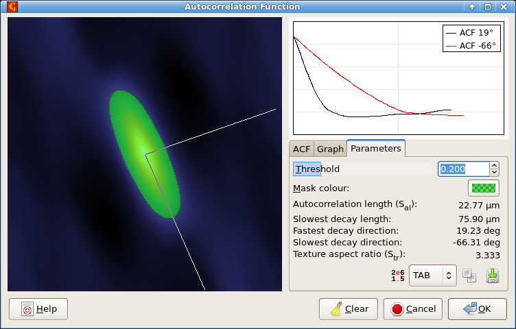
The full two-dimensional autocorrelation function introduced above is sometimes used to evaluate anisotropy of rough surfaces. The 2D ACF module calculates the function and can also plot its section in selected directions or calculate several roughness parameters that are based on 2D ACF.
Options in the ACF tab control how the function is calculated and displayed. In most cases the mean value should be subtracted before the calculation (as would Mean Zero Value do). This is selected by Mean value subtraction in Data adjustment. However, Plane levelling can be also useful. If you already adjusted the zero level correctly, select None to calculate the ACF from unaltered data. If there is a mask on the image the dialogue offers the standard masking options. See Masked Statistics Functions for an overview of masked ACF calculation.
The Graph tab contains settings for extracted ACF sections. They are the same as for normal profile extraction.
Finally, Parameters displays various numerical parameters derived from 2D ACF. They are determined from the decay of ACF in different directions and depend on Threshold, below which data points are considered essentially uncorrelated. The area above the selected threshold is marked using a mask on the ACF image.
The threshold is a fraction with respect to the maximum (occurring at the origin). In theoretical models the autocorrelation length corresponds to decay of ACF to 1/e. This is also the default value. However, in roughness standards it is usually chosen as 0.2. For comparable results, check that you use consistently one threshold value.
The autocorrelation length Sal is the shortest distance at which the ACF falls below the threshold. The corresponding direction is also shown, as well as the distance and direction of the slowest decay. The ration between the longest and smallest distances is the texture aspect ratio Str.
→ →
The full two-dimensional spectral density function is used to evaluate characteristic spatial frequencies occurring in surfaces. The 2D PSDF module calculates the function and can also plot its section in selected directions.
Options in the PSDF tab control how the function is calculated and displayed. Option Windowing selects the windowing type. If there is a mask on the image the dialogue offers the standard masking options. See Masked Statistics Functions for an overview of masked PSDF calculation.
The Graph tab contains settings for extracted PSDF sections. They are the same as for normal profile extraction.
Finally, Parameters displays some numerical parameters derived from 2D PSDF. Two are calculated using the angular spectrum, texture direction Std and texture direction index Stdi. Std is given by the direction in which the radial PSDF integral is the largest and determines the dominant texture direction. Stdi measures how dominant is the dominant direction by comparing the average over all directions to the dominant direction. Note that smaller Stdi means more spectral weight in the dominant direction (not less).


Several functions in → operate on two-dimensional slope (derivative) statistics.
calculates a plain two-dimensional distribution of derivatives, that is the horizontal and vertical coordinate on the resulting data field is the horizontal and vertical derivative, respectively. The slopes can be calculated as central derivatives (one-side on the borders of the image) or, if Use local plane fitting is enabled, by fitting a local plane through the neighbourhood of each point and using its gradient.
can also plot summary graphs representing one-dimensional distributions of quantities related to the local slopes and facet inclination angles given by the following formula:
Three different plots are available:
- , the distribution of the inclination angle ϑ from the horizontal plane. Of course, representing the slope as an angle requires the value and the dimensions to be the same physical quantity.
- is similar to the ϑ plot, except the distribution of the derivative v is plotted instead of the angle.
- visualises the integral of v2 for each direction φ in the horizontal plane. This means it is not a plain distribution of φ because areas with larger slopes contribute more significantly than flat areas.
function is a visualization aid that does not calculate a distribution in the strict sense. For each derivative v the circle of points satisfying
is drawn. The number of points on the circle is given by Number of steps.

→ →
This function can estimate the differential entropy of value and slope distributions and also provides a visualisation of how it is calculated.
The Shannon differential entropy for a probability density function can be expressed
where X is the domain of the variable x. For instance for the height distribution x represents the surface height and X is the entire real axis. For slope distribution x is a two-component vector consisting of the derivatives along the axes, and X is correspondingly the plane.
There are many more or less sophisticated entropy estimation methods. Gwyddion uses a relatively simple histogram based method in which the above formula is approximated with
where pi and wi are the estimated probability density, i.e. normalized histogram value, and width of the i-th histogram bin.
Of course, the estimated entropy value depends on the choice of bin width. With the exception of uniform distribution, for which the estimate does not depend on the bin size. From this follows that for reasonable distributions a suitable bin width is such that the estimated entropy does not change when the width changes somewhat. This is the criterion used for choosing a suitable bin width.
In practice this means the entropy is estimated over a large range of bin widths (typically many orders of magnitude), obtaining the scaling curve displayed in the graph on the right side of the dialogue. The entropy is then estimated by finding the inflexion point of the curve. If there is no such point, which can happen for instance when the distribution is too close to a sum of δ-functions, a very large negative value is reported as the entropy.
The entropies are displayed as unitless since they are logarithmic quantities. For absolute comparison with other calculations, it should be noted that in Gwyddion they are always calculated from quantities in base SI units (e.g. metres as opposed to for instance nanometres) and natural logarithms are used. The values are thus in natural units of information (nats).
The absolute entropy depends on the absolute width of the distribution. For instance, two Gaussian distributions of heights with different RMS values have different entropies. This is useful when we want to compare the absolute narrowness of structures in the height distribution. On the other hand, it can be useful to compare them in a manner independent on the overall scale. For this we can utilise the fact that the Gaussian distribution has the maximum entropy among all distributions with the same RMS value. The difference between this maximum and the estimated entropy is displayed as entropy deficit. By definition, it is always positive (apart from numerical issues).
[1] D. Nečas and P. Klapetek: One-dimensional autocorrelation and power spectrum density functions of irregular regions. Ultramicroscopy 124 (2013) 13-19, doi:10.1016/j.ultramic.2012.08.002
[2] D. Nečas, P. Klapetek and M. Valtr: Estimation of roughness measurement bias originating from background subtraction. Measurement Science and Technology (2020) 094010, doi:10.1088/1361-6501/ab8993
[3] D. Nečas, M. Valtr and P. Klapetek: How levelling and scan line corrections ruin roughness measurement and how to prevent it. Scientific Reports 10 (2020) 15294, doi:10.1038/s41598-020-72171-8
[4] D. Nečas: Self-consistent autocorrelation for finite-area bias correction in roughness measurement. Engineering Research Express 6 (2024) 025560, doi:10.1088/2631-8695/ad5302