Two-dimensional Fourier transform can be accessed using → → which implements the Fast Fourier Transform (FFT). Fourier transform decomposes signal into its harmonic components, it is therefore useful while studying spectral frequencies present in the SPM data.
The 2D FFT module provides several types of output:
- Modulus – absolute value of the complex Fourier coefficient, proportional to the square root of the power spectrum density function (PSDF).
- Phase – phase of the complex coefficient (rarely used).
- Real – real part of the complex coefficient.
- Imaginary – imaginary part of the complex coefficient.
and some of their combinations for convenience.
Radial sections of the two-dimensional PSDF can be conveniently obtained with 2D PSDF. Several other functions producing spectral densities are described in section Statistical Analysis. It is also possible to filter images in the frequency domain using one-dimensional and two-dimensional FFT filters or simple frequency splitting.
For scale and rotation-independent texture comparison it is useful to transform the PSDF from Cartesian frequency coordinates to coordinates consisting of logarithm of the spatial frequency and its direction. Scaling and rotation then become mere shifts in the new coordinates. The function → → calculates directly the transformed PSDF. The dimensionless horizontal coordinate is the angle (from 0 to 2π) the vertical is the frequency logarithm. It is possible to smooth the PSDF using a Gaussian filter of given width before the transformation.
Note that the Fourier transform treats data as being infinite, thus implying some cyclic boundary conditions. As the real data do not have these properties, it is necessary to use some windowing function to suppress the data at the edgest of the image. If you do not do this, FFT treats data as being windowed by rectangular windowing function which has really bad Fourier image thus leading to corruption of the Fourier spectrum.
Gwyddion offers several windowing functions. Most of them are formed by some sine and cosine functions that damp data correctly at the edges. In the following windowing formula table the independent variable x is from interval [0, 1] which corresponds to the normalized abscissa; for simplicity variable ξ = 2πx is used in some formulas. The available windowing types include:
| Name | Formula |
|---|---|
| None | 1 |
| Rect | 0.5 at edge points, 1 everywhere else |
| Hann | |
| Hamming | |
| Blackmann | |
| Lanczos | |
| Welch | |
| Nutall | |
| Flat-top | |
| Kaiser α | , where I0 is the modified Bessel function of zeroth order and α is a parameter |
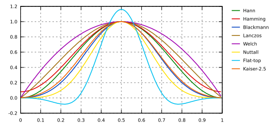
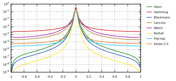
Envelopes of windowing functions frequency responses: Hann, Hamming, Blackmann, Lanczos, Welch, Nutall, Flat-top, Kaiser 2.5.

→ →
One excellent way of removing frequency based of noise from an image is to use Fourier filtering. First, the Fourier transform of the image is calculated. Next, a filter is applied to this transform. Finally, the inverse transform is applied to obtain a filtered image. Gwyddion uses the Fast Fourier Transform (or FFT) to make this intensive calculation much faster.
Within the 1D FFT filter the frequencies that should be removed from spectrum (suppress type: null) or suppressed to value of neighbouring frequencies (suppress type: suppress) can be selected by marking appropriate areas in the power spectrum graph. The selection can be inverted easily using the Filter type choice. 1D FFT filter can be used both for horizontal and vertical direction.

→ →
2D FFT filter acts similarly as the 1D variant (see above) but using 2D FFT transform. Therefore, the spatial frequencies that should be filtered must be selected in 2D using mask editor. As the frequencies are related to center of the image (corresponding to zero frequency), the mask can be snapped to the center (coordinate system origin) while being edited. There are also different display and output modes that are self-explanatory – image or FFT coefficients can be outputted by module (or both).

→ →
A simple alternative to 2D FFT filtering is the separation of low and high spatial frequencies in the image using a simple low-pass and/or high-pass filter. The frequency split module can create either the low-frequency or high-frequency image or both, depending on the selected Output type.
Cut-off selects the spatial frequency cut off, which is displayed as relative fraction of the Nyquist frequency and also as the corresponding spatial wavelength. If Edge width (again given as relative to Nyquist frequency) is zero the filter has sharp edge. For non-zero values the transition has the shape of error function, with specified width.
Frequency domain filtering can lead to artefacts close to image boundaries. Therefore, several boundary handling options are provided, aside from None which is mostly useful for periodic data (or otherwise continuous across edges). Laplace and Mirror extend the image by Laplace's equation method and mirroring, respectively, exactly as the Extend function. Smooth connect applies to rows and column the one-dimensional smooth extension method used in Roughness tool to suppress edge artefacts.