The wavelet transform is similar to the Fourier transform (or much more to the windowed Fourier transform) with a completely different merit function. The main difference is this: Fourier transform decomposes the signal into sines and cosines, i.e. the functions localized in Fourier space; in contrary the wavelet transform uses functions that are localized in both the real and Fourier space. Generally, the wavelet transform can be expressed by the following equation:
where the * is the complex conjugate symbol and function ψ is some function. This function can be chosen arbitrarily provided that it obeys certain rules.
As it is seen, the Wavelet transform is in fact an infinite set of various transforms, depending on the merit function used for its computation. This is the main reason, why we can hear the term “wavelet transform” in very different situations and applications. There are also many ways how to sort the types of the wavelet transforms. Here we show only the division based on the wavelet orthogonality. We can use orthogonal wavelets for discrete wavelet transform development and non-orthogonal wavelets for continuous wavelet transform development. These two transforms have the following properties:
- The discrete wavelet transform returns a data vector of the same length as the input is. Usually, even in this vector many data are almost zero. This corresponds to the fact that it decomposes into a set of wavelets (functions) that are orthogonal to its translations and scaling. Therefore we decompose such a signal to a same or lower number of the wavelet coefficient spectrum as is the number of signal data points. Such a wavelet spectrum is very good for signal processing and compression, for example, as we get no redundant information here.
- The continuous wavelet transform in contrary returns an array one dimension larger than the input data. For a 1D data we obtain an image of the time-frequency plane. We can easily see the signal frequencies evolution during the duration of the signal and compare the spectrum with other signals spectra. As here is used the non-orthogonal set of wavelets, data are highly correlated, so big redundancy is seen here. This helps to see the results in a more humane form.
For more details on wavelet transform see any of the thousands of wavelet resources on the Web, or for example [1].
Within Gwyddion data processing library, both these transforms are implemented and the modules using wavelet transforms can be accessed within → menu.

The discrete wavelet transform (DWT) is an implementation of the wavelet transform using a discrete set of the wavelet scales and translations obeying some defined rules. In other words, this transform decomposes the signal into mutually orthogonal set of wavelets, which is the main difference from the continuous wavelet transform (CWT), or its implementation for the discrete time series sometimes called discrete-time continuous wavelet transform (DT-CWT).
The wavelet can be constructed from a scaling function which describes its scaling properties. The restriction that the scaling functions must be orthogonal to its discrete translations implies some mathematical conditions on them which are mentioned everywhere, e.g. the dilation equation
where S is a scaling factor (usually chosen as 2). Moreover, the area between the function must be normalized and scaling function must be orthogonal to its integer translations, i.e.
After introducing some more conditions (as the restrictions above does not produce a unique solution) we can obtain results of all these equations, i.e. the finite set of coefficients ak that define the scaling function and also the wavelet. The wavelet is obtained from the scaling function as N where N is an even integer. The set of wavelets then forms an orthonormal basis which we use to decompose the signal. Note that usually only few of the coefficients ak are nonzero, which simplifies the calculations.
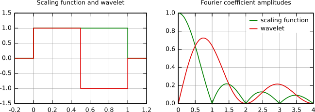
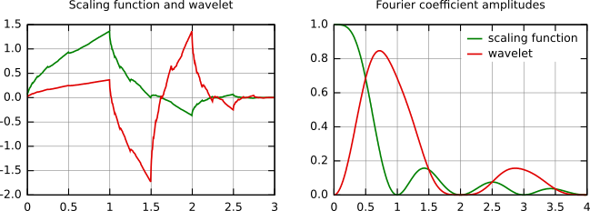
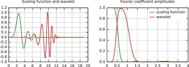
In the following figure, some wavelet scaling functions and wavelets are plotted. The most known family of orthonormal wavelets is the family of Daubechies. Her wavelets are usually denominated by the number of nonzero coefficients ak, so we usually talk about Daubechies 4, Daubechies 6, etc. wavelets. Roughly said, with the increasing number of wavelet coefficients the functions become smoother. See the comparison of wavelets Daubechies 4 and 20 below. Another mentioned wavelet is the simplest one, the Haar wavelet, which uses a box function as the scaling function.
There are several types of implementation of the DWT algorithm. The oldest and most known one is the Mallat (pyramidal) algorithm. In this algorithm two filters – smoothing and non-smoothing one – are constructed from the wavelet coefficients and those filters are recurrently used to obtain data for all the scales. If the total number of data D = 2N is used and the signal length is L, first D/2 data at scale L/2N - 1 are computed, then (D/2)/2 data at scale L/2N - 2, … up to finally obtaining 2 data at scale L/2. The result of this algorithm is an array of the same length as the input one, where the data are usually sorted from the largest scales to the smallest ones.
Within Gwyddion the pyramidal algorithm is used for computing the discrete wavelet transform. Discrete wavelet transform in 2D can be accessed using DWT module.
Discrete wavelet transform can be used for easy and fast denoising of a noisy signal. If we take only a limited number of highest coefficients of the discrete wavelet transform spectrum, and we perform an inverse transform (with the same wavelet basis) we can obtain more or less denoised signal. There are several ways how to choose the coefficients that will be kept. Within Gwyddion, the universal thresholding, scale adaptive thresholding [2] and scale and space adaptive thresholding [3] is implemented. For threshold determination within these methods we first determine the noise variance guess given by
where Yij corresponds to all the coefficients of the highest scale subband of the decomposition (where most of the noise is assumed to be present). Alternatively, the noise variance can be obtained in an independent way, for example from the AFM signal variance while not scanning. For the highest frequency subband (universal thresholding) or for each subband (for scale adaptive thresholding) or for each pixel neighbourhood within subband (for scale and space adaptive thresholding) the variance is computed as
Threshold value is finally computed as
where
When threshold for given scale is known, we can remove all the coefficients smaller than threshold value (hard thresholding) or we can lower the absolute value of these coefficients by threshold value (soft thresholding).
DWT denoising can be accessed with → → .

Continuous wavelet transform (CWT) is an implementation of the wavelet transform using arbitrary scales and almost arbitrary wavelets. The wavelets used are not orthogonal and the data obtained by this transform are highly correlated. For the discrete time series we can use this transform as well, with the limitation that the smallest wavelet translations must be equal to the data sampling. This is sometimes called Discrete Time Continuous Wavelet Transform (DT-CWT) and it is the most used way of computing CWT in real applications.
In principle the continuous wavelet transform works by using directly the definition of the wavelet transform, i.e. we are computing a convolution of the signal with the scaled wavelet. For each scale we obtain by this way an array of the same length N as the signal has. By using M arbitrarily chosen scales we obtain a field N×M that represents the time-frequency plane directly. The algorithm used for this computation can be based on a direct convolution or on a convolution by means of multiplication in Fourier space (this is sometimes called Fast Wavelet Transform).
The choice of the wavelet that is used for time-frequency decomposition is the most important thing. By this choice we can influence the time and frequency resolution of the result. We cannot change the main features of WT by this way (low frequencies have good frequency and bad time resolution; high frequencies have good time and bad frequency resolution), but we can somehow increase the total frequency of total time resolution. This is directly proportional to the width of the used wavelet in real and Fourier space. If we use the Morlet wavelet for example (real part – damped cosine function) we can expect high frequency resolution as such a wavelet is very well localized in frequencies. In contrary, using Derivative of Gaussian (DOG) wavelet will result in good time localization, but poor one in frequencies.
CWT is implemented in the CWT module that can be accessed with → → .
[1] Adhemar Bultheel: Learning to swim in a sea of wavelets. Bull. Belg. Math. Soc. Simon Stevin 2 (1995), 1-45, doi:10.36045/bbms/1103408773
[2] S. G. Chang, B. Yu, M. Vetterli: Adaptive wavelet thresholding for image denoising and compression. IEEE Trans. Image Processing 9 (2000) 1532–1536, doi:10.1109/83.862633
[3] S. G. Chang, B. Yu, M. Vetterli: Spatially adaptive wavelet thresholding with context modeling for image denoising. IEEE Trans. Image Processing 9 (2000) 1522–1531, doi:10.1109/83.862630