In practice objects exhibiting random properties are encountered. It is often assumed that these objects exhibit the self-affine properties in a certain range of scales. Self-affinity is a generalization of self-similarity which is the basic property of most of the deterministic fractals. A part of self-affine object is similar to whole object after anisotropic scaling. Many randomly rough surfaces are assumed to belong to the random objects that exhibit the self-affine properties and they are treated self-affine statistical fractals. Of course, these surfaces can be studied using atomic force microscopy (AFM). The results of the fractal analysis of the self-affine random surfaces using AFM are often used to classify these surfaces prepared by various technological procedures [1,2,3,4].
Within Gwyddion, there are different methods of fractal analysis implemented within → → .
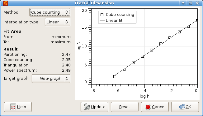
- Cube counting method [1,2]
- is derived directly from a definition of box-counting fractal dimension. The algorithm is based on the following steps: a cubic lattice with lattice constant l is superimposed on the z-expanded surface. Initially l is set at X/2 (where X is length of edge of the surface), resulting in a lattice of 2×2×2 = 8 cubes. Then N(l) is the number of all cubes that contain at least one pixel of the image. The lattice constant l is then reduced stepwise by factor of 2 and the process repeated until l equals to the distance between two adjacent pixels. The slope of a plot of log(N(l)) versus log(1/l) gives the fractal dimension Df directly.
- Triangulation method [1]
- is very similar to cube counting method and is also based directly on the box-counting fractal dimension definition. The method works as follows: a grid of unit dimension l is placed on the surface. This defines the location of the vertices of a number of triangles. When, for example, l = X/4, the surface is covered by 32 triangles of different areas inclined at various angles with respect to the xy plane. The areas of all triangles are calculated and summed to obtain an approximation of the surface area S(l) corresponding to l. The grid size is then decreased by successive factor of 2, as before, and the process continues until l corresponds to distance between two adjacent pixel points. The slope of a plot of log(S(l)) versus log(1/l) then corresponds to Df − 2.
- Variance (partitioning) method [3,4]
- is based on the scale dependence of the variance of fractional Brownian motion. In practice, in the variance method one divides the full surface into equal-sized squared boxes, and the variance (power of RMS value of heights), is calculated for a particular box size. The fractal dimension is evaluated from the slope β of a least-square regression line fit to the data points in log-log plot of variance as Df = 3 − β/2.
- Power spectrum method [3,4,5]
- is based on the power spectrum dependence of fractional Brownian motion. In the power spectrum method, every line height profiles that forms the image is Fourier transformed and the power spectrum evaluated and then all these power spectra are averaged. The factal dimension is evaluated from the slope β of a least-square regression line fit to the data points in log-log plot of power spectrum as Df = 7/2 + β/2.
- Structure function (HHCF) method
- is similar to the power spectrum method, but instead of the power spectrum, the structure function (height-height correlation function) is fitted around zero. The fractal dimension is evaluated from the slope β of a least-square regression line fit to the data points in log-log plot of variance as Df = 3 − β/2.
The axes in Fractal Dimension graphs always show already logarithmed quantities, therefore the linear dependencies mentioned above correspond to straight lines there. Frequently only a part of the plotted curve is a straight line as the end tend to be influenced by various systematic errors and artefacts. The measure of the axes should be treated as arbitrary.
Note that that results of different methods differ. This fact is caused by systematic error of different fractal analysis approaches.
Moreover, the results of the fractal analysis can be influenced strongly by the tip convolution. We recommend therefore to check the certainty map before fractal analysis. In cases when the surface is influenced a lot by tip imaging, the results of the fractal analysis can be misrepresented strongly.
Note, that algorithms that can be used within the fractal analysis module are also used in Fractal Correction module and Fractal Correction option of Remove Spots tool.
[1] C. Douketis, Z. Wang, T. L. Haslett, M. Moskovits: Fractal character of cold-deposited silver films determined by low-temperature scanning tunneling microscopy. Physical Review B 51 (1995) 11022, doi:10.1103/PhysRevB.51.11022
[2] W. Zahn, A. Zösch: The dependence of fractal dimension on measuring conditions of scanning probe microscopy. Fresenius J Analen Chem 365 (1999) 168-172, doi:10.1007/s002160051466
[3] A. Van Put, A. Vertes, D. Wegrzynek, B. Treiger, R. Van Grieken: Quantitative characterization of individual particle surfaces by fractal analysis of scanning electron microscope images. Fresenius J Analen Chem 350 (1994) 440-447, doi:10.1007/BF00321787
[4] A. Mannelquist, N. Almquist, S. Fredriksson: Influence of tip geometry on fractal analysis of atomic force microscopy images. Appl. Phys. A 66 (1998) 891-895, doi:10.1007/s003390051262
[5] W. Zahn, A. Zösch: Characterization of thin film surfaces by fractal geometry. Fresenius J Anal Chem 358 (1997) 119-121, doi:10.1007/s002160050360