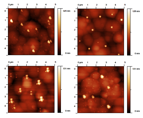
Tip convolution artefact is one of the most important error sources in SPM. As the SPM tip is never ideal (like delta function) we often observe a certain degree of image distortion due to this effect. We can even see some SPM tips imaged on the surface scan while sharp features are present on the surface.
We can fortunately simulate and/or correct the tip effects using algorithms of dilation and/or erosion, respectively. These algorithms were published by Villarubia (see [1]).
For studying the tip influence on the data we need to know tip geometry first. In general, the geometry of the SPM tip can be determined in several ways:
- Use manufacturer's specifications (tip geometry, apex radius and angle).
- Use scanning electron microscope of other independent technique to determine tip properties.
- Use known tip characterizer sample (with steep edges).
- Use blind tip estimation algorithm together with tip characterizers or other suitable samples.

→ →
Tip modelling implements the first approach. Using tip modelling most of the tips with simple geometries can be simulated. This way of tip geometry specification can be very efficient namely when we need to check only certainty map of perform tip convolution simulation.
The function offers several usual model shapes such as pyramids, cones or paraboloids. Each is described by a subset of the following parameters:
- Number of sides
The number of pyramid sides applies to pyramidal tips (which do not have a fixed number of sides by definition).
- Tip slope
Angle of the pyramid side, measured from the vertical plane. Small angles mean sharp tips and large angles means shallow tips.
- Tip rotation
Rotation with respect to a base orientation, measured anti-clockwise. It applies to tips which are not rotationally symmetric.
- Tip apex radius
Mean radius of curvature at the tip apex (applies to all tip shapes, except the delta-function). If the tip is not anisotropic, this is simply the radius of curvature in all directions.
- Tip anisotropy
Ratio expressing how much the tip is squashed along one of the two orthogonal directions with respect to the other. Only the elliptic parabola model has an anisotropy parameter.
The tip image dimensions are determined automatically using the source data to cover the data z-range.

→ →
To obtain more detailed (and more realistic) tip structure blind tip estimation algorithm can be used. Blind tip estimation algorithm is an extension of the well-known fact that on some surface data we can see images of certain parts of tip directly. The algorithm iterates over all the surface data and at each point tries to refine each tip point according to steepest slope in the direction between concrete tip point and tip apex.
We can use two modification of this algorithm within Gwyddion: partial tip estimation that uses only limited number of highest points on the image and full tip estimation that uses full image (and is much slower therefore). Within Gwyddion tip estimation module we can use also partial tip estimation results as starting point for full estimation. This improves the speed of full tip estimation.
The typical procedure is
- Use to start afresh, for instance after changing parameters.
- Run the partial estimation using .
- Run the full estimation using .
It is possible – and often useful – to run the full estimate with several topographical images in sequence. This can be achieved by selecting successively the images as Related data and running the estimation.
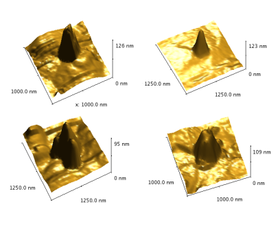
SPM tips obtained from data of previous figure using blind estimation algorithm.
The tip shape can change during the scanning. Therefore, it is sometimes useful to inspect how its blind estimation evolves with the scan lines. Of course, estimation from a single scan line is impossible. Hence, the image is split to horizontal stripes and the tip is estimated for each stripe.
The stripe-wise processing is enabled by Split to stripes, which also controls the number of stripes. You can choose which tip is displayed using Preview stripe. A tip radius graph is displayed below the preview – and can be created as output when Plot size graph is enabled. The function can also produce the full sequence of estimated tip images, which is enabled by Create tip images.


When we know tip geometry, we can use tip convolution (dilation) algorithm to simulate data acquisition process. For doing this use Dilation module ( → → ). This can be in particular useful when working with data being result of some numerical modelling (see e.g. [2]).
Note this algorithm (as well as the following two) requires compatible scan and tip data, i.e. the physical dimensions of a scan pixel and of a tip image pixels have to be equal. This relation is automatically guaranteed for tips obtained by blind estimate when used on the same data (or data with an identical measure). If you obtained the tip image by other means, you may need to resample it.
The opposite of the tip convolution is surface reconstruction (erosion) that can be used to correct partially the tip influence on image data. For doing this, use Surface Reconstruction function ( → → ). Of course, the data corresponding to points in image not touched by tip (e. g. pores) cannot be reconstructed as there is no information about these points.

As it can be seen, the most problematic parts of SPM image are data points where tip did not touch the surface in a single point, but in multiple points. There is a loss of information in these points. Certainty map algorithm can mark points where surface was probably touched in a single point.
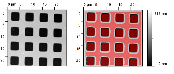
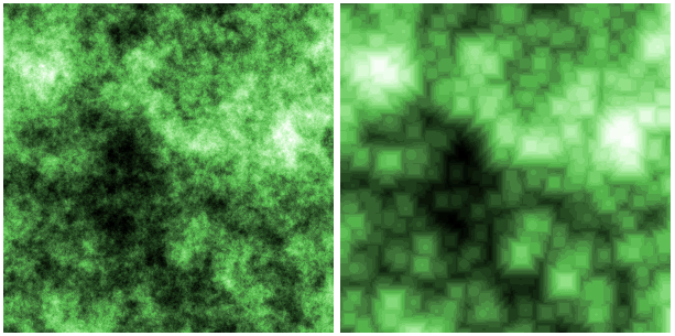
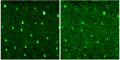
Certainty map obtained from standard grating. Note that the modelled tip parameters were taken from datasheet here for illustration purposes. (left) – sample, (right) – sample with marked certainty map.
Certainty map algorithm can be therefore used to mark data in the SPM image that are corrupted by tip convolution in an irreversible way. For SPM data analysis on surfaces with large slopes it is important to check always presence of these points. Within Gwyddion you can use Certainty Map function for creating these maps ( → → ).
[1] J. S. Villarrubia: Algorithms for Scanned Probe Microscope Image Simulation, Surface Reconstruction, and Tip Estimation. J. Res. Natl. Inst. Stand. Technol. 102 (1997) 425, doi:10.6028/jres.102.030
[2] P. Klapetek, I. Ohlídal: Theoretical analysis of the atomic force microscopy characterization of columnar thin films. Ultramicroscopy 94 (2003) 19–29, doi:10.1016/S0304-3991(02)00159-6