Value-reading and basic geometrical operations represent the core of any data processing program. Gwyddion offers a wide set of functions for data scaling, rotation, resampling or profile extraction. This section describes these simple but essential functions.
Most basic operations can be found in → menu; some are also carried out by tools.
Geometrical transformations in this group preserve pixels, i.e. a pixel in the transformed image corresponds precisely to one pixel in the source image. There is no interpolation.


Flip the data horizontally (i.e. about the vertical axis), vertically (i.e. about the horizontal axis) or around the diagonal (i.e. exchanging rows and columns) with → → , or , respectively.


Rotation of data by multiples of 90 degrees is done using some of the basic rotation functions: → → , or . Flipping both axes rotates the image by 180°.

The Crop tool can crop an image either in place or putting the result to a new image (with option Create new image). With Keep lateral offsets option enabled, the top left corner coordinates of the resulting image correspond to the top left corner of the selection, otherwise the top left corner coordinates are set to (0, 0).

→ →
Extending is essentially the opposite of cropping. Of course, adding more real data around the image borders is only possible by measuring more data. So this function offers, instead, several simple artificial extension methods such as mirrored and unmirrored periodic continuation or repetition of boundary values. The Laplace method works in the same way as Interpolate Data Under Mask and creates a smooth extension which converges to the mean value of the entire image boundary.
Transformations in this group do not map one pixel to one pixel and require interpolation.

→ →
Resample the data to different pixel dimensions (number of image columns and rows) using the selected interpolation method. The physical dimensions are unchanged.
If you want to specify the physical dimensions of one pixel, use Resample instead.

→ →
Upsample the data (along the axis with larger pixel size) to make pixels square. Most scans have pixels with 1:1 aspect ratio, therefore this function has no effect on them.
→ →
Resample the data to different physical pixel size using the selected interpolation method. The pixel size can be selected to match another image, which is required for some multi-data operations. The physical dimensions are unchanged.
If you want to specify the number of image rows and columns or scaling ratio, use Scale instead.

Function → → rotates the image by arbitrary angle. Unlike the simple geometrical transforms above, this requires interpolation, which can be specified in the dialogue.
After rotation, the image is no longer a rectangle with sides parallel to the axes. Option Result size specifies the area to take as the resulting image:
- Same as original preserves the image size, cutting off some data and adding some empty exterior data in the corners.
- Expanded to complete data ensures no parts of the image are cut off – which often means the results includes lots of empty exterior.
- Cut to valid data ensures the results contains no empty exterior – which often means cutting it considerably.
A mask can be optionally added over pixels corresponding to the exterior of the original image.

→ →
Binning is an alternative method of size reduction. The resulting image is not created by interpolating the original at given points but instead by averaging all original pixels contributing to the result pixel.
The rectangular block of pixels that are averaged is the bin. You can control its dimensions using Width and Height that are also downscaling factors in each direction. The origin of the first bin can be offset from the image origin. Note, however, that the result is formed only from complete bins; incomplete bins at image edges are ignored.
Trimmed mean can be used instead of the standard average, with Trim lowest and Trim highest controlling how many lowest and highest values are discarded before averaging. This can be useful for suppressing local outliers. When Sum instead of averaging is enabled, the resulting value is calculated as the sum of all the contributions. This would make little sense for typical topographical data. However, if the image represents a density-like quantity whose integral should be preserved, summing is the correct operation.
Functions in this group preserve pixels 1:1. However, they modify their values. See also the Arithmetic module which allows data manipulation using arithmetic expressions.


→ →
Data range can be limited by cutting values outside the specified range. The range can be set numerically or taken from the false colour map range previously set using the Colour range tool and it is also possible to cut off outliers farther than a chosen multiple of RMS from the mean value.

→ →
Periodic data, such as angles, are sometimes stored with an inconvenient wrap-around which makes them look discontinuous. For instance, the value range is from 0 to 360 degrees, but the data would be continuous if represented in range −180 to 180 degrees. Simple rewrapping then restores continuity.
The function has two parameters. Range is the value range (period in the z direction). Offset specifies the split value for rewrapping. The exact formula is
Symbols r and Δ represent the range and offset, respectively. Function fmod is the floating point modulo (remainder) function.

→ →
Change physical dimensions, units or value scales and also lateral offsets. This is useful for the correction of raw data that have been imported with wrong physical scales or as a simple manual recalibration of dimensions and values.
The recalibrations can be specified either as absolute, i.e. setting the dimensions or value range to given values, or as corrections applying a factor and/or offset. In addition a few special modes exist which can for instance match exactly the pixel size to another image.
Since settings are remembered between invocations, multiple images can be quickly recalibrated the same way. For new, unrelated recalibrations make sure the properties you do not want to change are set to Do not change or use the button.

The simplest value reading method is to place the mouse cursor over the point you want to read value of. The coordinates and/or value is then displayed in the data window or graph window status bar.

The Read Value tool offers more value reading possibilities: it displays coordinates and values of the last point of the data window the mouse button was pressed. It also displays a zoomed view of the image around this point.
The tool can average the values from a circular neighbourhood around the selected point, this is controlled by option Averaging radius. When the radius is 1, the value of a single pixel is displayed (as the simplest method does). Button shifts the surface to make the current z the new zero level.
Read Value can also display the inclination of the local facet or local surface curvature. Averaging radius again determines the radius of the area to use for the plane fit. Curvature in particular need relatively large areas to be reliable.
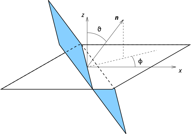
In all Gwyddion tools, facet and plane inclinations are displayed as the spherical angles (ϑ, φ) of the plane normal vector.
Angle ϑ is the angle between the upward direction and the normal, this means that ϑ = 0 for horizontal facets and it increases with the slope. It is always positive.
Angle φ is the counter-clockwise measured angle between axis x and the projection of the normal to the xy plane, as displayed on the following figure. For facets it means φ corresponds to the downward direction of the facet.

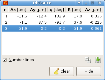
Distances and differences can be measured with the Distance tool. It displays the horizontal (Δx), vertical (Δy) and total planar (R) distances; the azimuth φ (measured identically to inclination φ ) and the endpoint value difference Δz for a set of lines selected on the data.
The distances can be copied to the clipboard or saved to a text file using the buttons below the list.

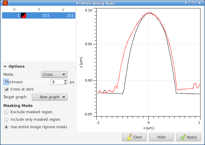
The Profiles along axes tool extracts scan lines in horizontal and/or vertical direction. The direction is controlled by Mode, which can be Horizontal, Vertical or Cross. In the cross mode both profiles are extracted simultaneously.
When the Cross at zero option is enabled, the profile abscissa origin is in the crossing point (or tick mark for horizontal and vertical profiles). This can be useful for alignment of profiles in the graph. When the option is disabled, the profile coordinates correspond to image coordinates in the corresponding direction.
Profiles can be of different “thickness” which means that multiple scan lines around the selected one are averaged. This can be useful for noise suppression while measuring regular objects. Profile thickness is denoted by line endpoint markers in the image.
Scan lines from multiple images can be simulatenously read using Multiprofile.

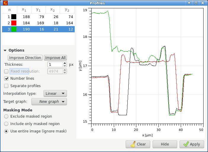
The Profile tool extracts profiles along arbitrary lines drawn and adjusted using mouse in the image, shown in a live preview in the dialogue. Profiles can be of different “thickness” which means that more neighbour data perpendicular to profile direction are used for evaluation of one profile point for thicker profiles. This can be very useful for noise suppression while measuring regular objects. Profile thickness is denoted by line endpoint markers in the image.
After profiles are chosen, they can be extracted to graphs (separate or grouped in one Graph window) for further analysis using Graph functions.
The profile curve is constructed from data sampled at regular intervals along the selected line. Values in points that do not lie exactly at pixel centres (which normally occurs for oblique lines) are interpolated using the chosen interpolation mode. Unless an explicit number of samples to take is set using the Fix res. option, the number of samples corresponds to the line length in pixels. This means that for purely horizontal or purely vertical lines no interpolation occurs.
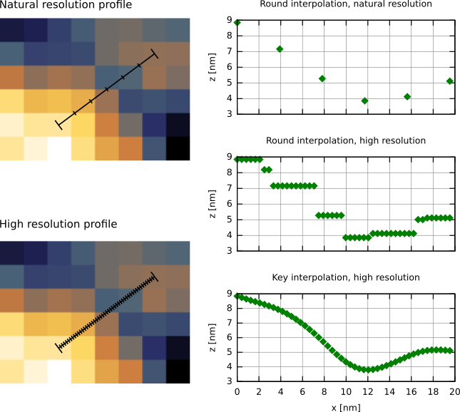
Illustration of data sampling in profile extraction for oblique lines. The figures on the left show the points along the line where the values are read for natural and very high resolution. The graphs on the right show the extracted values. Comparison of the natural and high resolution profiles taken with Round interpolation reveals that indeed natural-resolution curve points form a subset of the high-resolution points. The influence of the interpolation method on values taken in non-grid positions is demonstrated by the lower two graphs, comparing Round and Key interpolation at high resolution.
In the measurement of profiles across edges and steps, it is often important to choose the profile direction perpendicular to the edge. The buttons and can help with this. The first attempts to improve the orthogonality of the currently edited line, while the second tries to improve all selected lines. The line centres are preserved; only the directions of the profiles are adjusted. The automatic improvement is not infallible, but it usually works well for reasonably clean standalone edges.

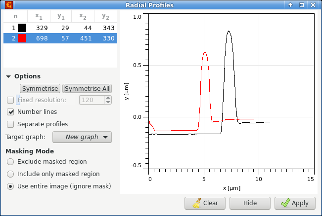
The Radial profile tool is somewhat similar to the standard profile tool. However, it does not extract profiles along lines. Instead, the line is used to define a circular area, with the centre marked by a tick. The extracted profile is then obtained by angular averaging. This is useful for extraction of the shapes of symmetrical surface features. The abscissa of the extracted graph is the distance from the centre instead of the distance along the line.
Although the line can be adjusted manually, finding the best centre for the radial profile manually may be difficult. Therefore, the tool can attempt a precise location of the best centre itself. You only need to select the line approximately and then press to adjust the currently edited line or to adjust all lines. The lines will be shifted slightly to minimise the differences between line profiles taken in different directions from the centre.


Function → → creates volume data from an image. The height field is interpreted as the surface of a solid object, as usual in AFM. Voxels below the surface (inside the material) are filled with 1s while voxels above the surface (outside) are filled with 0s. The z-coordinate of the volume data therefore corresponds to the image values, while the volume data values are unitless.
Function → → creates volume data from a sequence of images. All images in the file must have the same dimensions. They are then treated as planes in the volume data that are created by stacking the images. The z-coordinate of the volume data therefore corresponds to the stack index (and can be specified in the dialogue), while the volume data values have the same units as the image data.
Function → → creates XYZ data from an image. Each image pixel corresponds to one point in the created XYZ data. Therefore, the xy coordinates thus form a regular grid and all units are the same as for the image.
Function → → creates XYZ data from three images, one containing x coordinates, one y and one z. This is useful when the data were measured nominally on a regular grid, but the actual measurement locations differed from regular grid points and their coordinates were recorded in additional channels.