Most geometrical transformations, such as rotation, scaling or drift compensation utilize or depend on data interpolation. Also some other operations, e.g. profile extraction, can work with values between individual pixels and hence involve interpolation. Since SPM data are relatively coarsely sampled compared to measured details (full images are typically only a few hundred pixels in width and height), the interpolation method used can become critical for proper quantitative analysis of data properties. Gwyddion implements several interpolation methods [1] and the user can choose which method to use for most of the modules using interpolation.
Here, we describe the principles and properties of one-dimensional interpolation methods. All implemented two-dimensional interpolation methods are separable and thus simply composed of the corresponding one-dimensional methods. The following interpolation methods are currently available:
- Round
Round interpolation (also called nearest neighbourhood interpolation) is the simplest method – it just takes rounded value of the expected position and finds therefore the closest data value at integer position. Its polynomial degree is 0, regularity C-1 and order 1.
- Linear
Linear interpolation is a linear interpolation between the two closest data values. The value z at point of relative position x is obtained as
where z0 and z1 are values at the preceding and following points, respectively. Its polynomial degree is 1, regularity C0 and order 2. It is identical to the second-order B-spline.
- Key
Key interpolation (more precisely Key's interpolation with a = −1/2 which has the highest interpolation order) makes use also of values in the before-preceding and after-following points z-1 and z2, respectively. In other words it has support of length 4. The value is then obtained as
where
are the interpolation weights. Key's interpolation degree is 3, regularity C1 and order 3.
- Schaum
Schaum interpolation (more precisely fourth-order Schaum) has also support of length 4. The interpolation weights are
Its polynomial degree is 3, regularity C0 and order 4.
- NNA
Nearest neighbour approximation is again calculated from the closest four data values but unlike all others it is not piecewise-polynomial. The interpolation weights are
for k = -1, 0, 1, 2, where r-1 = 1 + x, r0 = x, r1 = 1 − x, r2 = 2 − x. Its order is 1.
- B-spline
The weights are
However, they are not used with directly function values as above, but with interpolation coefficients calculated from function values [1]. Its polynomial degree is 3, regularity C2 and order 4.
- O-MOMS
The weights are
However, they are not used directly with function values as above, but with interpolation coefficients calculated from function values [1]. Its polynomial degree is 3, regularity C0 and order 4.
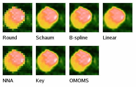
Illustration of the available interpolation types (the original pixels are obvious on the result of Round interpolation). All images have identical false colour map ranges.
[1] P. Thévenaz, T. Blu, M. Unser: Interpolation revisited. IEEE Transactions on medical imaging 10 (2000) 739–758, doi:10.1109/42.875199