Data Process → Level → Fix Zero

Data Process → Level → Zero Mean Value

The simplest functions that are connected with data levelling are Fix Zero and Zero Mean Value that just add a constant to all the data to move the minimum and mean value to zero, respectively.

Data Process → Level → Plane Level

Plane levelling is usually one of the first functions applied to raw SPM data. The plane is computed from all the image points and is subtracted from the data.

If a mask is present plane levelling offers to use the data under mask for the plane fitting, exclude the data under mask or ignore the mask and use the entire data.

The Three Point Levelling tool can be used for levelling very complicated surface structures. The user can simply mark three points in the image that should be at the same level, and then click Apply. The plane is computed from these three points and is subtracted from the data.

Data Process → Level → Facet Level

Facet Level levels data by subtracting a plane similarly to the standard Plane Level function. However, the plane is determined differently: it makes facets of the surface as horizontal as possible. Thus for surfaces with flat horizontal areas it leads to much better results than the standard Plane Level especially if large objects are present.

On the other hand, it is not suitable for some types of surface. These includes random surfaces, data with considerable fine noise and non-topographic images as the method does not work well if the typical lateral dimensions and “heights” differ by many orders.

Similarly to Plane Level, Facet Level can include or exclude the data under mask. This choice is offered only if a mask is present.

Finding the orientation of the facets is an iterative process that works as follows. First, the variation of local normals is determined:

where n_i is the vector of local facet normal (see inclination coordinates) in the i-th pixel. Then the prevalent normal is estimated as

where c = 1/20 is a constant. Subsequently, the plane corresponding to the prevalent normal n is subtracted and these three steps are repeated until the process converges. The gaussian weighting factors serve to pick a single set of similar local facet normals and converge to their mean direction. Without these factors, the procedure would obviously converge in one step to the overall mean normal – and hence would be completely equivalent to plain plane levelling.

Facet Level example: (a) uncorrected, sloping data; (b) data levelled by standard plane fitting (Plane Level); (c) data levelled by Facet Level.

Data Process → Level → Level Rotate

Level Rotate behaves similarly to Plane Level, however it does not simply subtract the fitted plane from the data. Instead, this module takes the fitted plane parameters and rotates the image data by a calculated amount to make it lie in a plane. So unlike Plane Level, this module should therefore preserve angle data in the image.

Data Process → Level → Polynomial Background

Fits data by a polynomial of the given degree and subtracts this polynomial. In the Independent degree mode the horizontal and vertical polynomial orders can be generally set separately, i.e. the fitted polynomial is

where m and n are the selected horizontal and vertical polynomial degrees, respectively. In the Limited total degree mode the fitted polynomial is

where n is the selected total polynomial degree.

Similarly to Plane Level, polynomial background subtraction can include or exclude the data under mask. This choice is offered only if a mask is present.

Data Process → Level → Flatten Base

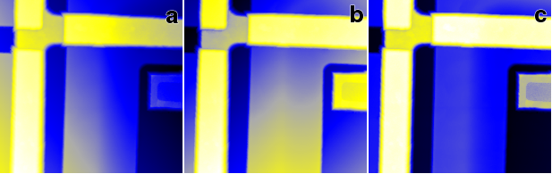
When a number of large features are present on a flat base surface the combination of masking, plane, facet and/or polynomial levelling can be used to level the flat base. It can require, however, several steps and trial and error parameter adjustment. Flatten Base attempts to perform this levelling automatically using a combination of facet and polynomial levelling with automated masking. It attempts to maximise the sharpness of the height distribution peak corresponding to the flat base surface.

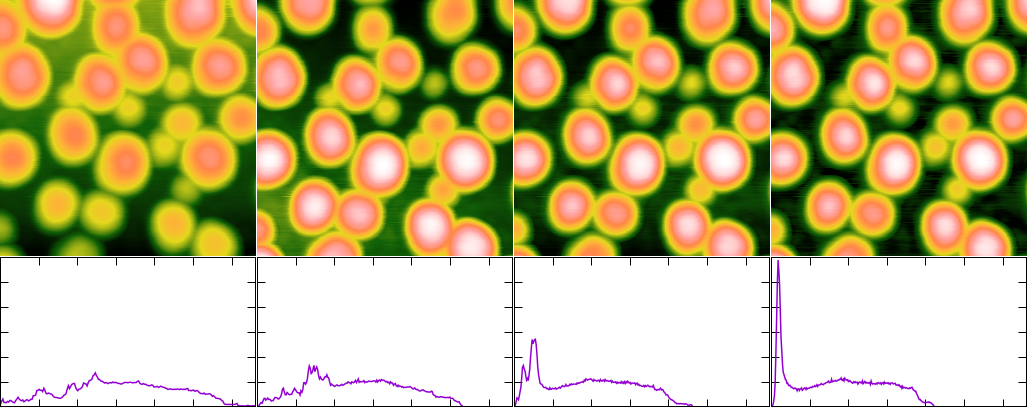
Flatten Base example: original image, levelled using Facet Level, levelled using Plane Level, levelled using Flatten Base. The original image is shown in linear colour scale, the levelled images are shown in adaptive colour scale. The graph below each image shows the corresponding height distribution (with the same axis ranges).

Data Process → Level → Revolve Arc

Data are levelled by revolving a virtual “arc” of given radius horizontally or vertically over (or under) the data. The envelope of this arc is treated as a background, resulting in removal of features larger than the arc radius (approximately). It is also possible to apply the levelling in both directions – in this case the arc is first revolved horizontally, then vertically.

By default the arc is revolved on the bottom side, preserving positive features (peaks). It is also possible to roll it on the top side by enabling Invert height.

Data Process → Level → Revolve Sphere

Data are levelled by revolving a virtual “sphere” of given over (or under) the data. The envelope of this sphere is treated as a background, resulting in removal of features larger than the sphere radius (approximately).

Data Process → Level → Median Level

The median levelling operation filters data with a median filter using a large kernel and treats the result as background. Only features smaller than approximately the kernel size will be kept.

Data Process → Level → Trimmed Mean

A more general variant of Median Level is the trimmed mean filter. In trimmed mean given fractions of lowest and highest values are discarded and the remaining data are averaged. For no discarded values the filter is identical to the mean value filter, whereas for the maximum possible number of discarded values (symmetrically) it becomes the median filter. The amount of discarded values can be given as a fraction (percentile) or as a specific number.

Data Process → Integral Transforms → Rank Filter

Another operation which generalises Median Level is the k-th rank filter. Imaging all the values in the neighbourhood of a pixel sorted, the median filter selects the value exactly in the middle. The k-th rank filter allows specifying any other rank or percentile to select at the filter output.

This means the filter can reproduce minimum, maximum and median filters – and anything between. It can also directly perform two rank filters simultaneously and calculating their difference. This is not useful for levelling, but allows for instance the calculation of local inter-quartile range for each pixel.