This section presents extended functions for correction (or creation) of global errors, such as low frequencies modulated on the data or drift in the slow scanning axis. Most of the functions described below deal with distortion purely in the xy plane – for instance Drift Compensation or Straighten Path. Some modify the value distribution (Coerce) or perform complex operations involving both coordinates and values.

→ →
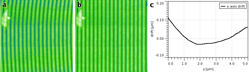
Compensate Drift calculates and/or corrects drift in the fast scanning axis (horizontal). This adverse effect can be caused by thermal effects or insufficient mechanical rigidity of the measuring device.
The drift graph, which is one of possible outputs, represents the horizontal shift of individual rows compared to a reference row (which could be in principle chosen arbitrarily, in practice the zero shift is chosen to minimize the amount of data sticking out of the image after compensation), with the row y-coordinate on the abscissa.
The drift is determined in two steps:
- A mutual horizontal offset is estimated for each couple of rows not more distant than Search range. It is estimated as the offset value giving the maximum mutual correlation of the two rows. Thus a set of local row drift estimations is obtained (together with the maximum correlation scores providing an estimate of their actual similarity).
- Global offsets are calculated from the local ones. At present the method is very simple as it seems sufficient in most cases: local drift derivatives are fitted for each row onto the local drift estimations and the global drift is then obtained by integration (i.e. summing the local drifts).
Option Exclude linear skew subtracts the linear term from the calculated drift, it can be useful when the image is anisotropic and its features are supposed to be oriented in a direction not paralled to the image sides.

→ →
Affine distortion in the horizontal plane caused by thermal drift is common for instance in STM. If the image contains a regular structure, for instance an atomic lattice of known parameters, the distortion can be easily corrected using this function.
The affine distortion correction requires to first select the distorted lattice in the image. This is done by moving the lattice selection on the preview with mouse until it matches the regular features present in the image. For images of periodic lattices, it is usually easier to select the lattice in the autocorrelation function image (2D ACF). Also, only a rough match needs to be found manually in this case. Button refines the selected lattice vectors to the nearest maxima in autocorrelation function with subpixel precision.
If scan lines contain lots of high-frequency noise the horizontal ACF (middle row in the ACF image) can be also quite noisy. In such case it is better to interpolate it from the surrounding rows by enabling the option Interpolate horizontal ACF.
The correct lengths of the lattice vectors a1 and a2 and the angle φ between them, entered to the dialogue, determine the affine transformation to perform. A few common lattice types (such as HOPG surface) are offered predefined, but it is possible to enter arbitrary lengths and angle.
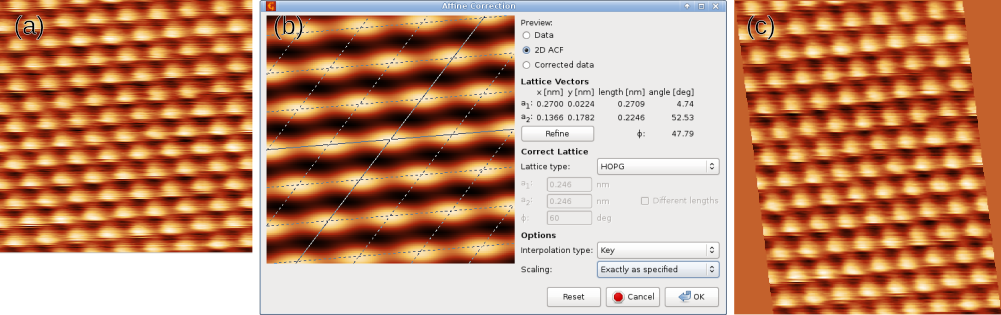
Affine correction example: (a) original image exhibiting an affine distortion, (b) correction dialogue with the lattice selected on the two-dimensional autocorrelation, (c) corrected image.
It should be noted that the correction method described above causes all lateral scale information in the image to be lost because the new lateral scale is fully determined by the correct lattice vectors. This is usually the best option for STM images of known atomic lattices, however, for a general skew or affine correction it can be impractical. Therefore, the dialogue offers three different scaling choices:
- Exactly as specified
Lattice vectors in the corrected image will have the specified lengths and angle between them. Scale information of the original image is discarded completely.
- Preserve area
Lattice vectors in the corrected image will have the specified ratio of lengths and angle between them. However, the overall scale is calculated as to make the affine transformation area-preserving.
- Preserve X scale
Lattice vectors in the corrected image will have the specified ratio of lengths and angle between them. However, the overall scale is calculated as to make the affine transformation preserve the original x-axis scale. This is somewhat analogous to the scale treatment in Drift compensation.
The function can also correct one image using the ACF calculated from another image (presumably a different channel in the same measurement) or apply the correction to all images in the file. The former is accomplished by selecting a different image as Image for ACF in the options. Affine transformation of all images in the file is enabled by Apply to all compatible images. Both options requite the other images to be compatible with the current one, i.e. having the same pixel and real dimensions.
→ →
Perspective distortion is unusual in scanning probe microscopy, but relatively common in other types of image data. The perspective distortion module can correct such distortion if the image contains features which are known to be in fact rectangular.
To apply the correction, a perspective rectangle is selected on the image by moving its four corners. The selected region is then transformed and extracted to the result. The preview can be switched between original and corrected data.
The module sets the pixel and physical dimensions of the result to estimated reasonable values, based on the assumption the distortion is not large. The dimensions then more or less correspond to the dimensions of the selected distorted rectangle in the original image. However, it is just an estimate. If the dimensions of the extracted rectangle can be determined more precisely, for instance using markings in the image, they should be set using Dimensions and Units.
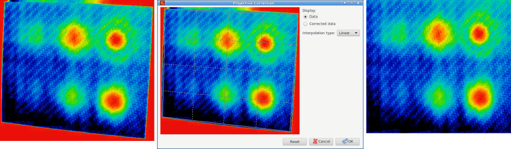
Perspective correction example. Left: original image exhibiting an perspective distortion. Centre: correction dialogue with the rectangle selected in the image. Right: corrected image.
Option Create new image controls whether the image is replaced with corrected or a new image created. The function can also apply the correction to all compatible images in the file.

→ →
General distortion in the horizontal plane can be compensated, or created, with Polynomial distortion. It performs transforms that can be expressed as
where Px and Py are polynomials up to the third total degree with user-defined coefficients. Note the direction of the coordinate transform – the reverse direction would not guarantee an unambiguous mapping.
The polynomial coefficients are entered as scale-free, i.e. as if the coordinate ranges were always [0, 1]. If Instant updates are enabled, pressing Enter in a coefficient entry (or just leaving moving keyboard focus elsewhere) updates the preview.

→ →
Extraction of data along circular features, curved step edges and other arbitrarily shaped smooth paths can be a useful preprocessing step for further analysis. Function creates a new image by “straightening” the input image along a spline path specified using a set of points on the image.
The points defining the path can be defined on the preview image. Each control point can be moved with mouse. Clicking into the empty space adds a new point, connected to the closer end of the path. Individual points can be deleted by selecting them in the point list in the left part of the dialogue and pressing Delete.
The shape of the extracted area is controlled by the following parameters:
- Thickness
The width of the extracted image, denoted by the perpendicular marks on the path. This is the full width, i.e. the distance to each side of the path is half of the thickness.
- Slackness
Parameter influencing the shape of the path between the control points. It can be visualised as the slackness of a string connecting the control points. For zero slackness the string is taut and the path is formed by straight segments. Increasing slackness means decreasing tensile stress in the string, up to slackness of unity for which the string is stress-free. Values larger than unity mean there is an excess string length, leading to compressive stress.
- Closed curve
If this option is enabled the path is closed, allowing the extraction of ring-shaped areas (for instance). Otherwise the path has two free ends.
Pressing computes a preview of the extracted image and shows it to the right of the input image. The preview is displayed vertically, with top edge corresponding to the path beginning and bottom edge to its end. The extracted image can be either oriented the same way or horizontally (from left to right), depending on Output orientation.
For certain combinations of path shape and thickness the resulting image can contain regions that lie outside the original image. Such regions are masked in the output and filled with a neutral value.
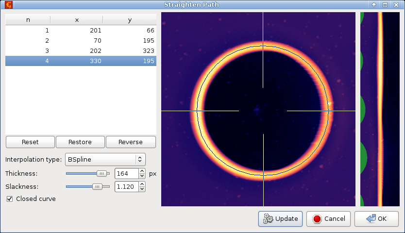
Straighten Path example, showing extraction of data along a closed circular path. The left part of the dialogue contains coordinates of the path-defining points and function options, the middle part shows the selected circular path (with perpendicular markers denoting the thickness), and the right part is a preview of the extracted straightened data.

→ →
Function Straighten Path stores the selected path with the data so that it can be recalled later. If you need the coordinates and/or directions corresponding to the straightened image for further processing you can use .
The function plots the real coordinates or tangents to the path, i.e. the direction cosines and sines, as graphs. Coordinates are selected as X position and Y position; directions are selected as X tangent and Y tangent. The number of points of each graph curve is the same as the number of rows of the straightened image created by Straighten Path and there is one-to-one correspondence between the rows and graph curve points.

→ →
Unrotate can automatically make principal directions in an image parallel with horizontal and/or vertical image edges. For that to work, the data need to have some principal directions, therefore it is most useful for scans of artificial and possibly crystalline structures.
The rotation necessary to straighten the image – displayed as Correction – is calculated from peaks in angular slope distribution assuming a prevalent type of structure, or symmetry. The symmetry can be estimated automatically too, but it is possible to select a particular symmetry type manually and let the module calculate only corresponding rotation correction. Note if you assume a structure type that does not match the actual structure, the calculated rotation is rarely meaningful.
It is recommended to level (or facet-level) the data first as overall slope can skew the calculated rotations.
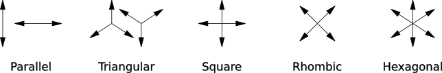
The assumed structure type can be set with Assume selector. Following choices are possible:
- Detected
Automatically detected symmetry type, displayed above as Detected.
- Parallel
Parallel lines, one prevalent direction.
- Triangular
Triangular symmetry, three prevalent directions (unilateral) by 120 degrees.
- Square
Square symmetry, two prevalent directions oriented approximately along image sides.
- Rhombic
Rhombic symmetry, two prevalent directions oriented approximately along diagonals. The only difference from Square is the preferred diagonal orientation (as opposed to parallel with sides).
- Hexagonal
Hexagonal symmetry, three prevalent directions (bilateral) by 120 degrees.
→ →
In periodic images, it can be useful to move the origin of the xy plane as it does not create any discontinuities. The same is true for images which may not be strictly periodic but, for instance, contain one dominant feature and are almost zero elsewhere.
The function moves a selected point in the image either to the centre or to the top-left corner, as specified with Move selected point to. The point coordinates can be entered numerically as Translation or by clicking in the preview image. Since the point is selected in the original image the second method is only possible when the original image is displayed (controlled by Display).
If the checkbox Update coordinate offsets is enabled the function adjusts the coordinate origin to preserve coordinates. Meaning an image feature will appear at the same coordinates after the transformation. Periodicity leads to some ambiguity here. In fact, there are infinite equally valid choices for the origin. The origin is chosen to avoid too large coordinates. When the checkbox is unchecked the lateral coordinates are kept unchanged.
Displacement field is a general method of image distortion in the xy plane. A vector is assigned to each point in the output image. This vector determines how far and in which direction to move from this point. The value found at the shifted position in the source image becomes the value of the pixel in the output image:
where v is the displacement vector.
The displacement field can be generated or obtained by several methods:
- Gaussian (scan lines)
The vectors have only the x component. The displacement is one-dimensional, along scan lines (image rows). It is a random Gaussian image, similar to Gaussian images generated by Spectral Synthesis.
- Gaussian (two-dimensional)
The vectors have both x and y components, so the displacement is two-dimensional. It is again a random Gaussian image.
- Tear scan lines
The vectors have only the x component. The displacement is one-dimensional, along scan lines (image rows). It is generated to tear segments of neighbour rows by shifting one to the left and another to the right. In the rest of the image the displacement is smooth (and close to zero) so continuity is preserved outside the tear.
- Image (scan lines)
The vectors have only the x component. The displacement is one-dimensional, along scan lines (image rows), and given by another image (selected as X displacement). The values of the image are directly used as the displacement vectors and must have the same units as lateral coordinates of the deformed image.
- Image (two-dimensional)
The vectors have both x and y components, so the displacement is two-dimensional. They are given by another images (selected as X displacement and Y displacement). The values of the images are directly used as the displacement vectors and must have the same units as lateral coordinates of the deformed image.

→ →
The module transforms the values in a height field to enforce certain prescribed statistical properties. The distribution of values can be transformed to Gaussian, with mean value and rms roughness preserved, or uniform, with minimum and maximum value preserved. It is also possible to enforce the same distribution as another height field selected as Template.
The transformation preserves the ordering of the values, i.e. if one point is higher than another before the transformation it will be also higher after the transformation. Option Data processing controls whether the transformation is applied to the image as a whole (Entire image) or each row separately, with the same distribution (By row (identically)). Note that in the latter case if a template is selected each row of the transformed image will have the same value distribution (approximately) as the template.
In addition, a different kind of transformation can be performed, discretisation of the values into given number of levels. This operation is selected with Discrete levels. There are two different discretisations available, either the height levels are equidistant from minimum to maximum value (Uniform) or they are calculated so that after the transformation each level will consist of approximately the same number of pixels (Same area).
→ →
Radial smoothing processes the image with a Gaussian smoothing filter, but in polar coordinates. This function is useful for images which should be relatively smooth and exhibit radial symmetry.
The image can be smoothed either along radial profiles – with Gaussian filter width controlled by Radius – or angularly along arcs of constant radius from the centre – with width controlled by Angle. The transformation to polar coordinates and back does not preserve the image perfectly. Subtle (and occasionally less subtle) artefacts can occur, in particular close to the centre, even with no actual smoothing.