Many of the Gwyddion data processing modules produce graph as an output. Graphs can be exported into text files or further analysed within Gwyddion by several graph processing modules. These modules can be found in the Graph menu in the Gwyddion main window. Note that the number of graph modules is quite limited now and consists of basic modules for doing things that are very frequent within SPM data analysis. For more analytical tools you can use your favourite graph processing program.
In this section the graph modules present in Gwyddion are briefly presented.


First of all zooming and data reading functions are available directly in the graph window:
- Logarithmic axes – horizontal and vertical axes can be switched between linear and logarithmic using the logscale buttons. Switching to logarithmic scale is possible only for positive values (either on abscissa or ordinate).
- Zoom in and zoom out – after selecting zoom in simply draw the area that should be zoomed by mouse. Zoom out restores the state where all data can be seen.
- Measure distances – enables user to select several points within the graph and displays their distances and angles between them.
Graph Flip flips the graph vertically. In other words the ordinate is inverted, whereas the abscissa is kept untouched. The functions directly modifies the curve data; it does not just change the presentation.
Graph Invert flips the graph horizontally. In other words the abscissa is inverted, whereas the ordinate is kept untouched. The functions directly modifies the curve data; it does not just change the presentation.

Graph Cut is a very simple module that cuts graph curves to the selected range (either given numerically or on the graph with mouse) and creates a new graph. If Cut all curves all curves are cut and put to the new graph; otherwise just the one chosen curve.

Graph level is also a simple module that currently performs linear fit of each graph curve and subtracts the fitted linear functions from them.

Graph align shifts the graphs curves horizontally to maximise their mutual correlations, i.e. match common features in the curves. This is useful in particular for comparison of profiles taken in different locations.
Two simple functions combine data of all curves to one, which is added to the plot. They differ slightly by data averaging approach.
- simply collects the data from all curves. It only merges two data points if the abscssae are the same, averaging the ordinates. The resulting curve thus usually oscillates between points belonging to the input curves if they are slightly vertically shifted.
- attempts to combine close points, averaging both ordinates and abscissae. Usually the resulting curve has a similar (or somewhat larger) number of points to one input curve, not all of them together. It should be also much smoother than for the simple merge, although sometimes there can be still visible oscillations.
The graph window controls allow switching between linear and logarithmic axes. However, for the fitting of power-law-like dependencies it is often useful to physically transform the data by taking logarithms of the values. The logscale transform graph function performs such transformation. You can choose which axis to transform (x, y or both), what to do with non-positive values if they occur and the logarithm base. A new graph is then created, with all curves transformed as requested.


Graph curve data can be exported to text files using . The export dialogue allows choosing several style variations that particular other software may find easier to read. Options Export labels, Export units and Export metadata allow adding informational lines before the actual data. This can be very useful for reminding what the file contains, but may cause problems when the file is read in other software.
Option POSIX number format enforces standard machine-readable scientific number format with decimal dot. Otherwise the values are written according to locale settings (office-style software may like that; scientific software generally does not).
The other important option that influences the structure of the entire file is Single merged abscissa. By default individual curves are written to the file sequentially, separated by empty lines. When this checkbox is enabled the curve export writes one multi-column table with data of all curves and a single abscissa in the first column. If the curves are not sampled identically, some rows will of course contain values only for some curves. Exported file with two separated curves can look like
0.1 3.32e6
0.2 3.80e6
0.4 4.15e6

0.0 11.1
0.3 9.66
0.4 9.70
while with single merged abscissa the same data would be saved
0.0 --- 11.1
0.1 3.32e6 ---
0.2 3.80e6 ---
0.3 --- 9.66
0.4 4.15e6 9.70
It is also possible to export a vector (EPS) or bitmap (PNG) rendering of the graph using or . However, these options are rather rudimentary. Gwyddion is not a dedicated plotting software and if you want nice graphs use one instead – for instance gnuplot or matplotlib.

Graph statistics display summary information about entire graph curves or selected ranges. The dialogue shows two main groups of quantities that are calculated differently.
Simple Parameters are calculated from the set of ordinate values, without any regard to abscissae. This is important to keep in mind when the curve is sampled non-uniformly, i.e. the intervals between abscissae differ, possibly a lot. A part of the curve which is sampled more densely contains relatively more points and thus also influences the result more. The available parameters include elementary characteristics with the same meaning as for two-dimensional data. Several of them also coincide with basic roughness parameters calculated by the Roughness tool.
On the other hand, Integrals are obtained by integration, utilising the trapezoid rule (or a similar approximation). Therefore, longer intervals contribute more to the results. Available quantities include:
- Projected length
- The length of the selected interval (or the entire abscissa range if no interval is selected).
- Developed length
- Sum of lengths of linear segments connecting curve points.
- Variation
- Integral of absolute value of the derivative – calculated as the sum of absolute values of ordinate differences.
- Average value
- Area under the curve divided by the projected length.
- Area under curve
- The total integral (sum of positive and negative area).
- Positive area
- Integral of portions of the curve where it is positive.
- Negative area
- Integral of portions of the curve where it is negative.
- Root mean square
- Integral of squared values divided by the projected length.
One-dimensional statistical functions are calculated for graphs using the same definitions as for images. They are described in the Statistical Functions tool documentation. The available functions include height and angle distributions, autocorrelation function, height-height correlation function and spectral density. They can be calculated for the selected curve or for all curves at once if All curves is enabled.
A major difference between images and graphs is that graph curves do not need to have uniformly spaced abscissa values (uniform sampling). In such case the curve is resampled within the calculation of the statistical functions to uniform sampling. The default sampling step is such that the number of points is preserved. However, it can be modified by Oversampling which gives how many more points the resampled curve should have compared to the graph curve. Occasionally it may be useful to use oversampling larger than 1 even for regularly sampled graph curves.

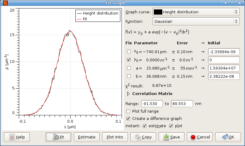
The curve fitting is designed namely for fitting of statistical functions used in roughness parameters evaluation. Therefore most of the available functions are currently various statistical functions of surfaces with Gaussian or exponential autocorrelation functions. Nevertheless it also offers a handful of common general-purpose functions. See the list of fitting functions.
Within the fitting module you can select the area that should be fitted (with mouse or numerically), try some initial parameters, or let the module to guess them, and then fit the data using Marquardt-Levenberg algorithm.
As the result you obtain the fitted curve and the set of its parameters. The fit report can be saved into a file using button. Pressing button adds the fitted curve to the graph, if this is not desirable, quit the dialogue with .

The module for fitting of force-distance curves is very similar to the general curve fitting module, it is just specialized for force-distance curves. Currently, the module serves for fitting jump-in part of force-distance curve (representing attractive forces) using different models:
- van der Waals force between semisphere and half-space
- van der Waals force between pyramid and half-space
- van der Waals force between truncated pyramid and half-space
- van der Waals force between sphere and half-space
- van der Waals force between two spheres
- van der Waals force between cone and half-space
- van der Waals force between cylinder and half-space
- van der Waals force between paraboloid and half-space
Note that the curve being fitted must be a real force-distance curve, not a displacement-distance or sensor-distance curve. Recalculation of cantilever deflection into force should be done before calling this module.
Also note that for small cantilever spring constants the amount of usable data in attractive region is limited by effect of jumping into contact.

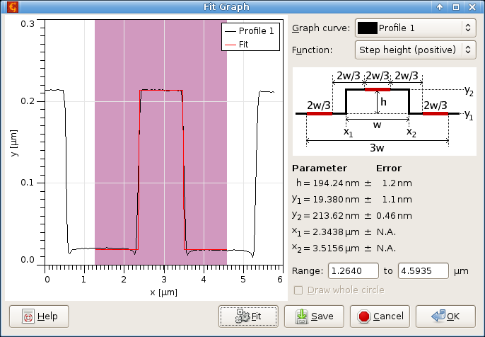
Critical dimension module can be used to fit some “typical” objects that are often found while analysing profiles extracted from microchips and related surfaces. These objects are located in the graph and their properties are evaluated.
The user interface of this module is practically the same as of the graph fit module.

DOS spectrum module intended to obtain Density-of-States spectra from I-V STM spectroscopy. It calculates
and plots it as graph.

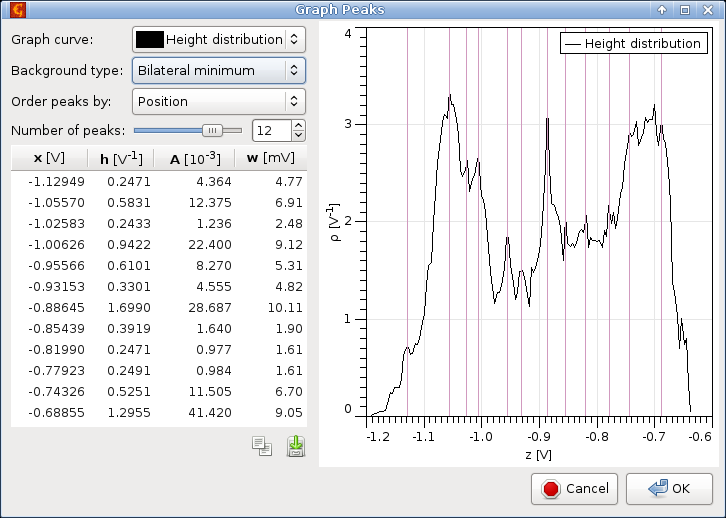
The most prominent peaks in graph curves can be automatically located with subsample precision. You can specify the number of most prominent peaks as Number of peaks and the function will mark them on the graph. Peak prominence depends on its height, area and distance from other peaks. Usually the function's idea what are the most prominent peaks agrees quite well with human assessment. If you disagree with the choice you can ask for more peaks and ignore those you do not like. It is also possible for locate negative peaks, i.e. valleys, by enabling option Invert (find valleys).
A table of all the peaks is displayed in the left part, sorted according to Order peaks by. Ordering by position means peaks are listed as they are displayed on the graph from left to right. Prominence order means more significant peaks are listed first.
Several basic characteristics are displayed for each peak: position (abscissa) x, height h, area A, and width (or variance) w. The position is calculated by quadratic subpixel refinement of the peak maximum. The remaining quantities depend on how the peak background is defined. Possible choices include Zero meaning peaks base is always considered to be zero, and Bilateral minimum meaning the peak background is a step function passing through the nearest curve minima on the left and right side of the peak.

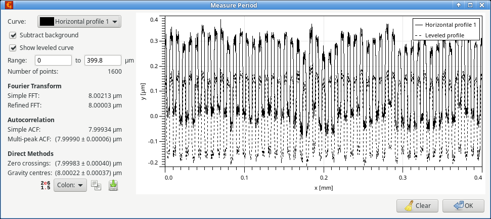
Many methods for measurement of the period/pitch of periodic profiles such as gratings have been proposed. The graph period measurment module implements several of them (see reference [1] for their description). For reasonably well measured gratings all the good methods
- Refined Fourier transform
- Multi-peak ACF
- Zero crossings
- Gravity centres
should give comparable results, although they differ in sensitivity to various artefacts in the data. Refined Fourier transform is the most robust for odd shapes of the repeating unit. However, it does not provide any error estimate.
Two elementary methods are also included, simple Fourier transform and simple ACF, which just find the position of the main peak in the power spectrum or ACF. They should not be used for evaluation and are present mainly for completness.
If the profile has been already correctly levelled and the zero line selected, the function can evaluate the profile without any preprocessing. Otherwise, Subtract background should be checked to enabled background removal based on a robust procedure (see again [1]). In such case Show levelled curve can be used to display the preprocessed profile alongside with the unmodified data.

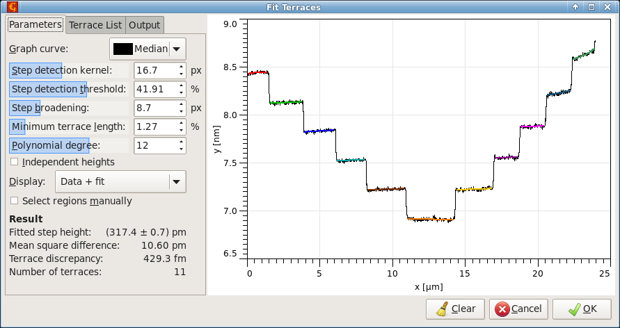
Terrace or amphitheatre-like structures can be measured using one-dimensional profiles, similarly as they are measured from image data in Terraces. The graph and image modules are almost identical. Therefore, the following only highlights the main differences:
Step detection kernel and broadening are one-dimensional. They are still measured in pixels – which correspond to average spacing between curve points. Minimum terrace area is replaced by minimum length, measured as the fraction of the total abscissa range.
There is no masking option. Instead, terraces can be marked manually on the graph using mouse when Select regions manually is enabled.
There is an additional choice in Display menu, Step detection. It shows the results of the edge detection filters and marks the selected threshold using a dashed red line. This is one of the most useful graphs for parameter tuning.
Pixel area Apx is replaced with Npx, the number of curve points the terrace consists of.
[1] D. Nečas, A. Yacoot, M. Valtr, P. Klapetek: Demystifying data evaluation in the measurement of periodic structures. Measurement Science and Technology 34 (2023) 055015, 10.1088/1361-6501/acbab3