Elementary operations with volume data include:

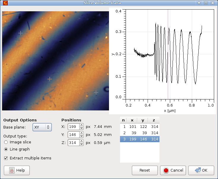
Profiles along any axis and image slices in planes orthogonal to any axis can be extracted with Volume Data → Cut and Slice.

The image slice in the selected plane, called Base plane, is always shown in the left part and the profile along the remaining orthogonal axis is shown in the right part of the dialogue. You can change the where the line profile is taken by moving the selected point in the image. Conversely, the image plane location can be moved by selecting a point in the profile graph. Both can be also entered numerically as X, Y and Z (in pixel coordinates).

You can choose between image and profile extraction freely by changing Output type. Changing the output type only influences whether the module creates the image on the left or the profile graph on the right when you press OK.

It is also possible to take multiple profiles or image slices at the same time. If Extract multiple items is enabled a list of selected points will appear on the right. In this case the output type influences the selection. In the Image slice mode you can select only one point in the image (determining the profile shown in the graph) but multiple points in the graph, each determining one output image plane. Conversely, in the Line graph mode you can select only one point in the graph (determining the image plane shown) but multiple points in the image, determining where the line profiles will be taken.

Switching betwen the output types when mutli-item extraction is enabled reduces the selected coordinate set to a single point. You can also use the Reset button to reduce the selection to the default single point if you want to start afresh.

Screenshot of the Cut and Slice volume data processing module, showing the simultaneous extraction of three line profiles along the z-axis.

Volume data can be exported to text files in several formats using Volume Data → Export Text. The possible output formats are

Basic overall characterisation of profiles along the z-axis can be performed using Volume Data → Summarize Profiles. This function creates an image formed by statistical characteristics of profiles taken along the z-axis. The set of available statistical quantities is the same as in the Row/column statistics tool.

The dual image/graph selection generally works very similarly to Image and profile extractions. The main difference is that an interval can be selected in the graph, defining the part of the image stack from which the statistical characteristics will be calculated. The interval can be also entered numerically using the Range entries.

The image on the left shows the calculated characteristics and corresponds to the output of the module. Selecting a different point in the image changes the profile displayed in the graph, which can be useful for choosing a suitable range. The value for the selected profile is displayed below the statistical quantity selector. However, choosing a profile does not influence the output in any way.

Basic overall characterisation of xy planes can be performed using Volume Data → Summarize Planes. This function creates a graph formed by statistical characteristics of individual xy-planes in the volume data or their parts. The set of available quantities is a subset of those calculated by Statistical quantities tool. A few quantities can take some time to calculate for all layers.

The dual image/graph selection generally works very similarly to Image and profile extractions. The main difference is that a rectangular region can be selected in the image plane, defining a rectangle from which the statistical characteristics will be calculated. The rectangle can be also entered numerically using the Origin and Size controls.

The graph on the right shows the calculated characteristics and corresponds to the output of the module. Selecting a different position in the graph changes the xy plane displayed in the image, which can be useful for choosing a suitable region. The value for the selected plane is displayed below the statistical quantity selector. However, choosing a plane does not influence the output in any way.

Arithmetic with volume data works exactly the same as image data arithmetic, including the same expression syntax.

The preview shows the average over all levels and the set of automatic variables is slightly different:

Techniques of imaging spectroscopy like F-D in QNM (Quantitative Nanomechanical Mapping) applications, I-V in semiconductor engineering, Raman in material characterization require to measure spectrum per each point of data grid on sample surface. Working with obtained array is not so simple, as we need to work with thousands of spectra and analyze each of them. If the sample of interest has limited number of regions with very similar spectra inside each region, some technique grouping similar spectra together can be of great help. One possible way of doing so is using clustering analysis. In Gwyddion currently two methods is implemented: K-means and K-medians.

Both algorithms are intended to find K clusters with similar spectra inside the cluster and maximally different between clusters. So Number of clusters is how many clusters K you want to obtain in the result. Convergence precision digits and Max. iterations regulate convergence criteria of algorithms that stop either if required precision of cluster centers position is achieved or allowed number of convergence cycles is exceeded. Higher precision require more steps to achieve, second limit is mostly intended to get rid of endless loops if the precision is to high for this set of data.

Normalize is somewhat experimental technique that qives nice results for imaging spectroscopy. If you are not interested in spectral intensities and want to cluster data by similarity of middle-frequencies of spectral features (it is typical, for example, for Raman microscopy), than enable this checkbox. It removes low frequency background by substraction of minimum withing the moving window, and then normalizes spectrum to make average intensity be equal 1.0. Both modules outputs two datafields: one shows to which cluster belongs the current spectrum, another shows error — difference between the current spectrum and center of corresponding cluster. If normalization is enabled than third datafield shows values the spectral intensities was divided by during normalization (after low-freq. filtering). Also graph with spectra corresponding to the centers of clusters is extracted.

Algorithms beside this two modules are based on usual unsupervized learning clustering: K-means and K-medians, correspondingly. We consider each spectrum (graph extracted along z-axis) to be the point in multidimensial space with the number of dimensions equal number of data point in the graph. We define distance between points as square root from sum of squared differencies along each direction (L²-norm). Than we initialize both algorithms by choosing random K points from the volume data as cluster centers. Than the usual two step algorithm is applied: we assign each point to the cluster whose center is nearest to the point and then move centers of the clusters. The difference between two modules is how to calculate the cluster center: it is mean value of cluster points for K-means and median along each direction for K-medians. The results from the last iteration are returned back to the program.

Remove outliers for K-means modifies algorithm for calculation of cluster centers to include only datapoints within Outliers threshold multiplied by data variation σ for each cluster. It removes single distinct bogus data points (like spikes, cosmic rays in Raman spectroscopy and so on) from calculation, making cluster centers somewhere more clean and distinct and also can shift border between intermixing clusters to more correct place between two centers of maximal point densities not disturbed by far outliers.

A few volume data functions are dedicated to MFM data processing. They are generally analogous to their image counterparts.

Conversion of MFM data to force gradient is exactly the same for volume and image data. Therefore, the summary of image MFM data conversion applies to volume data unchanged.

The transfer function estimation Volume Data → Transfer Function Guess is also quite similar to image transfer function estimation. The TF is estimated for each level in the volume data and its various properties plotted as graphs. Which graphs are plotted can be selected in the Output Options tab. The regularisation parameter σ can be the same for all levels, or it can be estimated for each level by enabling Estimate sigma for each level. The computation then takes notably longer. For the Least squares method, even the transfer function size can be estimated for each level when Estimate size for each level is enabled. The size given in the dialogue then determines the size of the output – and thus maximum possible size. Smaller transfer functions are extended with zeros to this size.

The stray field consistency check Volume Data → Stray Field Consistency recalculates the field to a different height similarly to MFM field shift. However, since the volume data contains images corresponding to many different levels, it is possible to calculate the field for each and compare it to the calculated field. And this is what the module does.