Volume data can be also used to represent stacks of images, i.e. coming from high-speed Scanning Probe Microscopy, representing multiple measurements of the sample, either on the same place or when moving laterally. In this case the data should be loaded as stack of images along the z axis. Such data can be processed by specialized functions available in the menu of the toolbox, mostly described in this part of the User Guide. On top of it, the general functions for handling Volume data can be used as well.
A few simple corrections or adjustments can be applied automatically to each xy plane in the volume data.
→ → applies plane levelling to each plane. In other words, it subtracts the mean plane from all images formed by xy planes. Each plane is treated separately.
→ → applies plane levelling using the same plane, the mean one, to each plane in the image stack. It calculates a single mean plane from all the images formed by xy planes, and subtracts the mean plane from all the images.
→ → applies facet leveling to all the images formed by xy planes, see description of the Facet Level algorithm for more details. Each plane is treated separately.
→ → applies flatten base algorithm to all the images formed by xy planes, see description of the Flatten Base algorithm fro more details. Each plane is treated separately.
→ → applies step line correction algorithm to all the images formed by xy planes, see description of the Step Line Correction module for images. Each plane is treated separately.
→ → replaces the outliers in each xy plane by the mean value of this plane. Outliers are defined here as values lying farther than three standard deviations from the mean.
→ → performs 1D FFT filtering in each xy plane. The power spectrum shown in the graph can be calculated for every plane individually, or it can be averaged from all the planes. By changing the preview level, one can go through all the planes and cross-check the filtering impact. Mouse selection in the graph and the suppression methods have same logic as in the 1D FFT Filtering module for images.
→ → performs detection and removal of scars (fast scanning axis feedback loop errors) in each xy plane. Each plane is treated separately and preview z level can be used to go through them. Scars detection method is same as in the Mark Scars module for images.
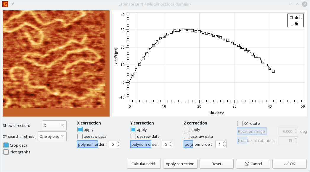
→ → performs detection and removal of drift in each xy plane. Drift is detected by cross-correlation which can be applied either to adjacent planes, one by one, which is optimal for larger drifts observed during the image stack acquisition, or an average plane can be used as a reference, which is optimal for small drifts or noisy data. Preview z level can be used to go through the planes, including visualisation of the cropped data after application of drift correction. On top of XYZ drift estimation, the images can be also rotated in given range, searching for the rotation angle which gives the best correlation score.
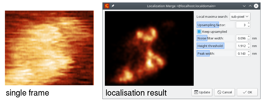
When multiple images of the same surface area are measured and the image stack is stored as Volume data, they can be used for a super-resolution image calculation, e.g. using some hypothesis about sample statistical parameters.
→ → performs the localisation algorithm [1]. At every xy plane the local peaks are detected, a probability for peak location is expressed and summed across the planes. The method works best on biomolecules or similar objects consisting of resolvable peaks, lying on a flat surface, and can remove the tip convolution impact and provide a high resolution image from series of low resolution ones. An important assumption is that the tip touches slightly different parts of the object at each scan, making the method well suited to soft samples in liquid environment. Note that the individual frames have to be aligned to display the same area of the surface, for this, e.g. the Estimate Drift module can be used.
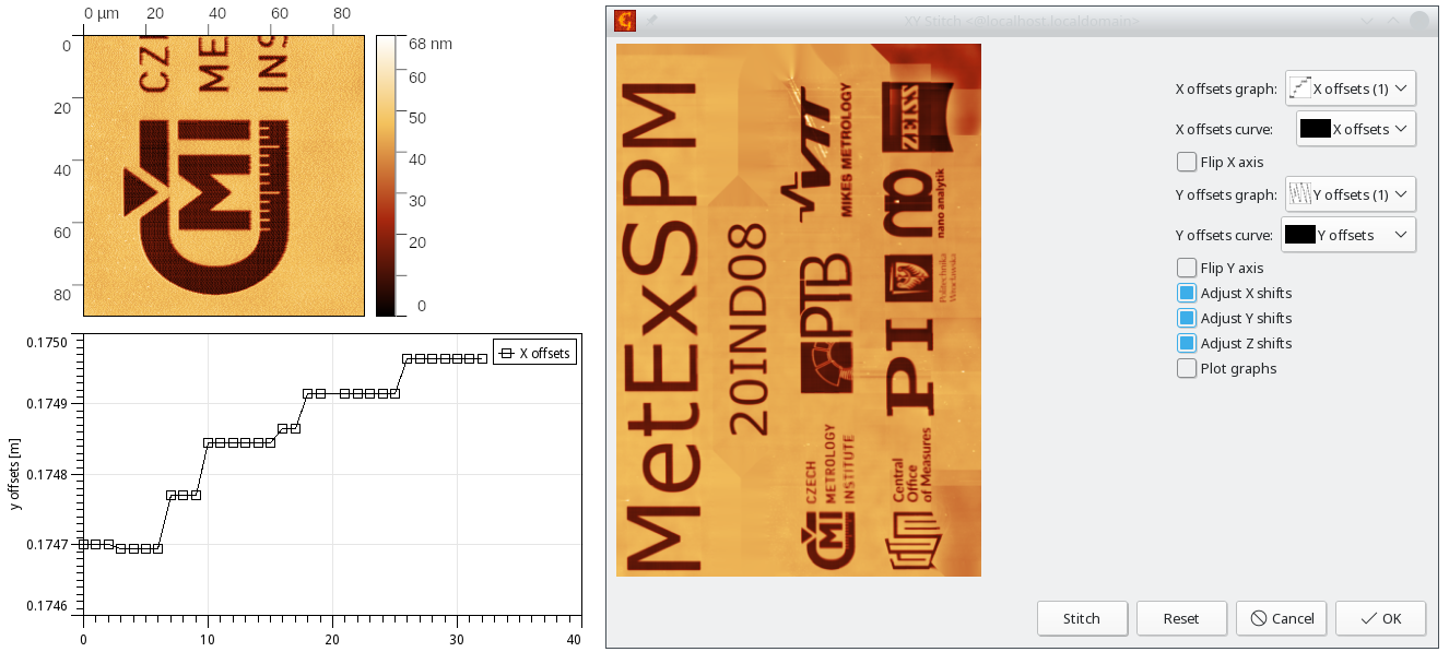
When the image stack represents different areas on the surface, a merged data representing larger area of the surface can be created. For this an information coming from sample coarse motion stage or from detected image overlaps can be used.
→ → performs stitching of a set of images represented as volume data, using the overlaps to minimize mutual offsets and using graphs of X and Y translations between the images. The X and Y translations are in base units (i.e. usually meters) and its X axis is treated as the frame number.
[1] G.R Heath, E. Kots, J.L. Robertson, et al.: Localization atomic force microscopy. Nature 594 (2021) 385–390, 10.1038/s41586-021-03551-x