The XYZ data processing possibilities are currently rather limited. Most analysis has to be done after their conversion to an image – the basic type of data for which Gwyddion offers plenty of functions.
Basic XYZ data operations currently include merging of two point sets, available as → . Merging can avoid creation of points at exactly the same lateral coordinates. Instead, their values are averaged – this is enabled by Average coincident points.

→
Gwyddion excels at working with data sampled in a regular grid, i.e. image data. To apply its data processing functions to irregular XYZ data, such data must be interpolated to a regular grid. In other words, rasterized.
Several interpolation methods are available, controlled bu the Interpolation type option:
- Round
This interpolation is analogous to the Round (nearest neighbour) interpolation for regular grids. The interpolated value in a point in the plane equals to the value of the nearest point in the XYZ point set. This means the Voronoi tessellation is performed and each Voronoi cell is “filled” with the value of the nearest point.
- Linear
This interpolation is analogous to the Linear interpolation for regular grids. The interpolated value in a point is calculated from the three vertices of the Delaunay triangulation triangle containing the point. As the tree vertices uniquely determine a plane in the space, the value in the point is defined by this plane.
- Field
The value in a point is the weighted average of all the XYZ point set where the weight is proportional to the inverse fourth power of the mutual distance. Since all XYZ data points are considered for the calculation of each interpolated point this method can be very slow.
- Average
Ad hoc method obtaining pixel values using a combination of simple averaging and propagation. In dense locations where many XYZ points fall into a single pixel the value assigned to such pixel is a sort of weighted mean value of the points. In sparse locations where relatively large regions contain no XYZ data points the pixel value is propagated from close pixels that contain some XYZ data points. The main feature of this interpolation type is that it is always fast while often producing quite an acceptable result.
The first two interpolation types are based on Voronoi tessellation and Delaunay triangulation that is not well-defined for point sets where more than two points lie on a line or more than three lie on a circle. If this happens the triangulation can fail and an error message is displayed.
The values outside the convex hull of the XYZ point set in the plane are influenced by Exterior type:
- Border
The point set is not amended in any manner and the values on the convex hull simply extend to the infinity.
- Mirror
The point set is amended by points “reflected” about the bounding box sides.
- Periodic
The point set is amended by periodically repeated points from around the opposite side of bounding box.
The horizontal and vertical pixel dimensions of the resulting image are specified as Horizontal size and Vertical size in the Resolution section.
Often resulting image should have square pixels. This can be achieved by pressing button . The function does not try to enforce square pixels during the resolution and range editing to avoid changing values that you in fact want to keep. So you always need to make the pixels square explicitly.
It is possible to rasterize only a portion of the XYZ data and also render a part of their exterior. The region to render to image is controlled by the ranges specified in the Physical Dimensions section of the dialogue. Button sets the region to a rectangle containing the XYZ data completely. It is also possible to select the region to render on the preview, of course provided that it lies inside the currently displayed region.
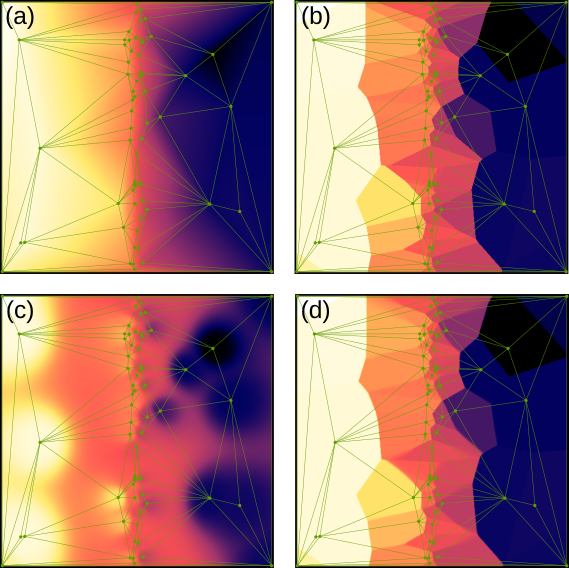
Delaunay triangulation displayed on top of (a) Linear, (b) Round, (c) Field and (d) Average interpolations of an irregular set of points. Since the points are sparse, Average interpolation is quite similar to Round, only a bit blurred.
If the XYZ data represent an image, i.e. the points form a regular grid oriented along the Cartesian axes with each point in a rectangular region present exactly once, the rasterization function can directly produce the corresponding image. This is done using button that appears at the top of the dialogue in this case.


→
→
The basic function is exactly the same as Fix Zero for image data. It shifts all values to make the minimum equal to zero.
removes the mean plane. It offers two methods. Subtraction is completely analogous to Plane Level for image data and consists in simple subtraction of the mean plane which is found using ordinary least-squares method.
Rotation removes the mean plane by true rotation of the point cloud, an operation exactly possibly only with XYZ data (the corresponding Level Rotate for images is approximate). Furthermore, the function ensures that the mean plane is horizontal after rotation, which corresponds to removal of mean plane in the total least-squares sense. Of course, since rotation mixes lateral coordinates and data values, it is only possible when z is the same physical quantity as x and y (presumably length).
Rotation changes the x and y point coordinates, potentially making the XYZ data incompatible with other data in the file. By enabling Update X and Y of all compatible data you can update the lateral coordinates of all other XYZ data sets in the file to match the lateral coordinates in the current one after rotation. The z values of the other data are, of course, kept intact.

→
This function is also available for images. See Fit Shape for images for differences between the image and XYZ variants.
Least-squares fitting of geometrical shapes and other predefined functions to the entire data can serve diverse purposes: removal of overall form such as spherical surface, measurement of geometrical parameters or creation of idealised data matching imperfect real topography. It is also possible to use the module for generation of artificial data if nothing is fitted and all the geometrical parameters are entered explicitly, altough this still requires providing input data that define the XY points.
The basic usage requires choosing the type of shape to fit, selected as Function type (see the description of fitting shapes), and pressing the following three buttons in given order:
Automatic initial estimate of the parameters. Usually the initial estimate is sufficient to proceed with fitting. When it is too off it may be necessary to adjust some of the parameters manually to help the least-squares fitting find the correct minimum. For some functions the estimation uses a randomly chosen subset of the input data to avoid taking too much time. Hence it is non-deterministic and pressing the button again can result in a somewhat different initial parameter estimate.
Least-squares fit using a randomly chosen subset of the input data. For large input data it is much faster than the full fit but in most cases it will converge to parameters quite close to final. It allows checking quickly whether the least-squares method is going to converge to the expected minimum – and simultaneously getting the parameters values closer to this minimum for the subsequent full fit.
Full least-squares fit using the entire data. This can take some time, especially for large input data and functions that are slow to evaluate.
The residual mean square difference per input point is displayed below the tabs as Mean square difference. It is recalculated whenever the preview is recalculated, so not only after fitting but also after estimation and manual adjustments.
The basic controls in the first tab also allow selecting the output from the fitting, which can be either the fitted shape, the difference between input data and fitted shape, or both.
The preview image can show either the input data, the fitted shape or the difference between the two – which is usually the most useful option. The difference can be displayed with an adapted color map in which red color means the input data are above the fitted shape and blue color means the input data are below the fit. This is enabled with Show differences with adapted color map.
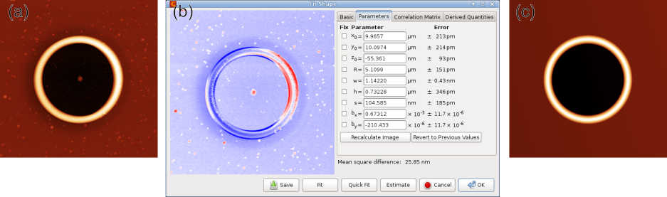
Shape fitting example: (a) original topographial data of a ring structure on the surface of a thin film, (b) fitting dialog with parameters on the right side and difference between data and fit displayed in the left part, (c) resulting fitted shape.
The Parameters tab displays the values of all fitting parameters and their errors and allows their precise control. Each parameter can be free or fixed. Fixed parameters are not touched by any estimation or fitting function; they are kept at the value you entered. When you change parameter value manually the preview is not recalculated automatically – press to update it. Button allows returning to the previous parameter set. For estimation, fitting or manual manipulation this means the set of parameter values before the operation modified them. For reverting it means the parameter set before reverting – so pressing the button repeatedly alternates between the last two parameter sets.
Tab Correlation Matrix displays, after a successful fit, the correlation matrix. Correlation coefficients that are very close to unity (in absolute value) are highlighted.
Finally, tab Derived Quantities displays various useful values calculated from fitting parameters. Some functions have no derived quantities, some have several. Most derived quantities represent parameters that you may be interested in more than in the actual fitting parameters but that are unsuitable as fitting parameters due to problems with numerical stability. The derived quantities are displayed with error estimates, calculated using law of error propagation (including parameter correlations).
A typical example is the curvature of spherical surface versus its radius of curvature. While the radius is more common it goes from infinity to negative infinity when the surface changes between convex and concave (i.e. is very close to flat), making it unsuitable as a fitting parameter. In contrast, curvature is zero for a flat surface. Therefore, curvature is used as the fitting parameter and the radius of curvature is displayed as a derived quantity.