Data Process → Measure Features → Curvature

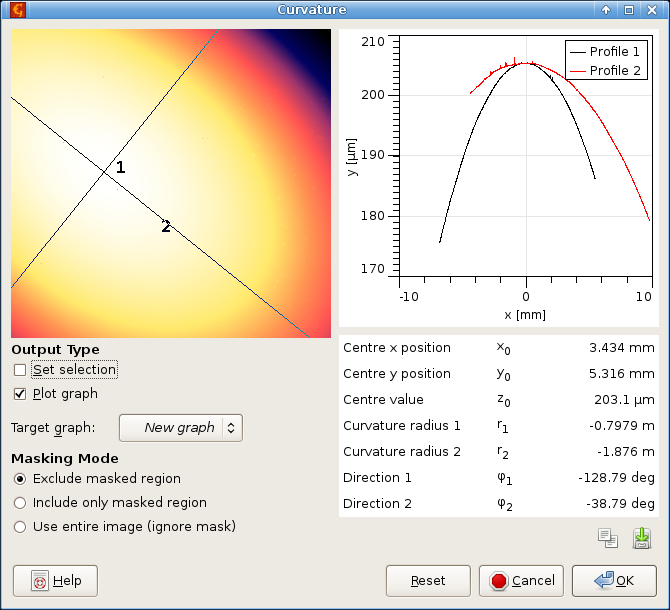
The global surface curvature parameters are calculated by fitting a quadratic polynomial and finding its main axes. Positive signs of the curvature radii correspond to a concave (cup-like) surface, whereas negative signs to convex (cap-like) surface, mixed signs mean a saddle-like surface.

Beside the parameter table, it is possible to set the line selection on the data to the fitted quadratic surface axes and/or directly read profiles along them. The zero of the abscissa is placed to the intersection of the axes.

Similarly to the background subtraction functions, if a mask is present on the data the module offers to include or exclude the data under mask.

Curvature dialogue screenshot showing the strong deflection of a glass plate with a thin film with compressive internal stress.

Data Process → Measure Features → Fit Shape

Form removal as well as measurement of geometrical parameters can be performed by fitting geometrical shapes on the data using the least-squares method. The Fit Shape module is essentially the same for images and XYZ data and it is described in detail in the XYZ data processing part. Only the differences are mentioned here.

Standard masking is supported for images. That is if a mask is present the dialogue offers to use the data under the mask, exclude the data under mask or ignore the mask and use the entire data. Since the excluded pixels can be outliers or image parts not conforming to the chosen shape it it possible to avoid them also in the difference image by disabling Calculate differences for excluded pixels.

Data Process → Measure Features → Facet Analysis

Facet analysis enables to interactively study orientations of facets occurring in the data and mark facets of specific orientations on the image. The top left view displays data with preview of marked facets. The smaller bottom left view, called facet view below, displays the two-dimensional slope distribution.

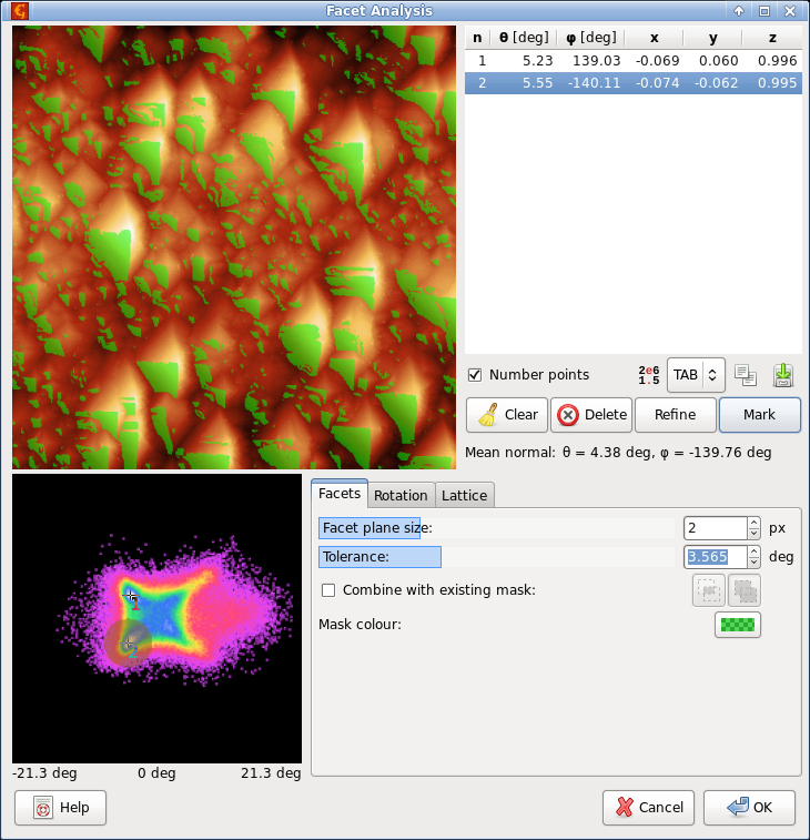
Facet analysis screenshot, showing two selected points on the angular distribution and marked facets for one of them.

The centre of facet view always correspond to zero inclination (horizontal facets), slope in x-direction increases towards left and right border and slope in y-direction increases towards top and bottom borders. The exact coordinate system is a bit complex (an area preserving transformation between spherical angles and the planar facet view is used) and it adapts to the range of slopes in the particular data displayed. The range of inclinations is displayed below the facet view.

Points selected on the facet view, i.e. directions in space, are listed in the top right corner as both angles and unit vector components. You can also choose the direction of the selected point by clicking on the image view. The direction is then set to the local facet at that position in the image.

Standard controls allowing manipulation with the entire list or the selected point are below the list. Button Refine tries to improve the position of selected point to a local maximum in the facet view. Button Mark creates a mask on the image corresponding to the selected direction and a range of close directions. The directions are simultaneously shown on the facet view. The mean normal of the selected region is displayed as Mean normal below.

The bottom right part contains tabs with settings and some advanced operations.

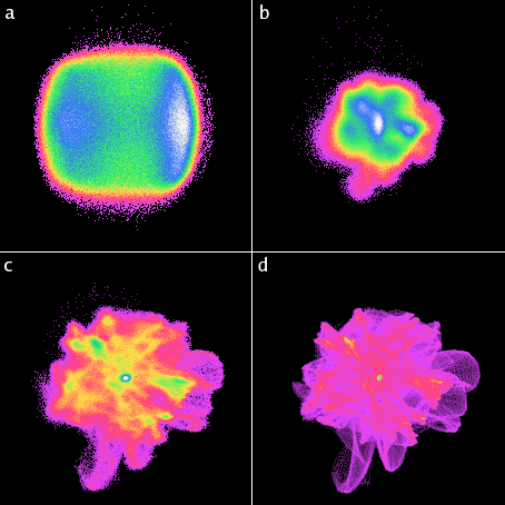
Illustration of the influence of fitted plane size on the distribution of a scan of a delaminated DLC surface with considerable fine noise. One can see the distribution is completely obscured by the noise at small plane sizes. The neighbourhood sizes are: (a) 0, (b) 2, (c) 4, (d) 7. The angle and false colour mappings are full-scale for each particular image, i.e. they vary among them.

Data Process → Measure Features → Facet Measurement

Facet measurement allows to interactively select and mark several facets of specific orientations on the image, measure their positions and store the results in a table. The top left view displays data with preview of marked facets. The smaller bottom left view, called facet view below, displays the two-dimensional slope distribution.

The centre of facet view always correspond to zero inclination (horizontal facets), slope in x-direction increases towards left and right border and slope in y-direction increases towards top and bottom borders. The exact coordinate system is a bit complex (an area preserving transformation between spherical angles and the planar facet view is used) and it adapts to the range of slopes in the particular data displayed. The range of inclinations is displayed below the facet view.

Facet plane size controls the size (radius) of plane locally fitted in each point to determine the local inclination. The special value 0 stands for no plane fitting, the local inclination is determined from symmetric x and y derivatives in each point. The choice of neighbourhood size is crucial for meaningful results: it must be smaller than the features one is interested in to avoid their smoothing, on the other hand it has to be large enough to suppress noise present in the image.

Tolerance determines the range of directions for marking. It also determines the search range for refining the the selected direction.

The currently selected point in facet view (facet orientation) is displayed as Selected ϑ and φ . Button Refine tries to improve the position of selected point to a local maximum in the facet view. Button Mark creates a mask on the image corresponding to the selected direction and a range of close directions. If Instant facet marking is enabled facets are marked immediately as the selected point changes (the Mark button is then disabled).

Once you are satisfied with the facet selection press Measure to add a measurement to the table below. Each row of the table contains

The mean normals are calculated by simple averaging of the unit normal vectors n, which is appropriate when their spread is relatively small. The standard deviation is calculated in radians as follows

where bar denotes the mean normal.

Data Process → Measure Features → Lattice

Parameters of regular two-dimensional structures can be obtained by analysing data transformed into a form that captures their regularity. The ACF and PSDF are particularly well-suited for this because they exhibit peaks corresponding to the Bravais lattice vectors for the periodic pattern.

Peaks in the two-dimensional ACF correspond to lattice vectors in the direct space (and their integer multiples and linear combinations). Peaks in the two-dimensional PSDF correspond to lattice vectors of the reciprocal lattice. The matrices formed by the lattice vectors in direct and frequency space are transposed inverses of each other. With a suitable transformation either can be used to measure the lattice.

The Gwyddion function Measure Lattice can utilise either ACF or PSDF for the measurement. Since regular lattices with large periods correspond to peaks in the ACF image that are far apart but peaks in the PSDF that are close, it is preferable to use the ACF in this case to improve the resolution. Conversely, the PSDF image is more suitable if the lattice periods are small. In the dialogue you can switch freely between direct and frequency space representations and the selected lattice is transformed as necessary.

If scan lines contain lots of high-frequency noise the horizontal ACF (middle row in the ACF image) can be also quite noisy. In such case it is better to interpolate it from the surrounding rows by enabling the option Interpolate horizontal ACF.

The button Estimate attempts to find automatically the lattice for the image. When it does not select the vectors as you would like you can adjust the vectors in the image manually. The selection can be done either in a manner similar to Affine Distortion (this corresponds to choosing Show lattice as Lattice), or only the two vectors can be shown and adjusted (Vectors). Either way, when you choose approximately the peak positions, pressing the Refine button adjusts the positions of the vectors to improve the match with the peaks. Button Reset can be used to restore the vectors to a sane initial state.

The lattice vectors are always displayed as direct-space vectors, with components, total lengths and directions. The angle shown as φ is the angle between the two vectors.

The direct lattice vectors a₁ and a₂ are related to the reciprocal lattice vectors b₁ and b₂ by the following relation:

where R denotes a 90 degree rotation matrix. The inverse transform is similar. Therefore, the lattice vectors must always be considered as a pair. Changing for instance b₁ in the PSDF image changes both a₁ and a₂.

Sometimes it is useful to measure a single lattice vector, e.g. in images of one-dimensional periodic structures. The second vector then gets in the way. For this there exists a single-vector mode, enabled by Measure single vector. It hides the second vectors and ensures a₁ are b₁ are parallel and with mutually reciprocal lengths, as expected.

Data Process → Measure Features → Terraces

Terrace measurement can be used either to measure steps between plateaus in terrace or amphitheatre-like structures, or calibration by measuring such structures with precisely known step heights – in particular atomic steps on silicon [1].

The image processing has several parts:

Some of them are optional. Furthermore, filtering and segmentation is interactive, whereas fitting is only run when button Fit is pressed. Intermediate results can be visualised by choosing the image to display using the Display menu. At the beginning, the most useful image is usually Marked terraces which shows individual recognised terraces in different colours.

Parameter Step detection kernel of edge detection is the same as for the Gaussian step filter. The following parameters control segmentation:

Segmentation can be augmented – or replaced – by a user-supplied mask. If the image has a mask, the standard masking options are offered. Here Exclude masked region means excluding it from the detected terraces. This allowing prevention of unwanted terrace merging – for instance by drawing manually small pieces of the boundaries using Mask Editor tool.

If option Do not segment, use only mask is enabled, no filtering is done and the mask is directly used as marked terraces (or their edges, depending on the masking mode). Filtering of terraces by area is still applied.

The total degree of the two-dimensional polynomial to fit is determined by parameter Polynomial degree. The polynomial is constructed in the same manner as in Polynomial levelling with limited total degree, except for the different base heights of each terrace.

The subsequent processing depends on whether Independents heights is enabled. If terrace heights are independent, each detected terrace is allowed to have arbitrary height offset. The module does not attempt to fit the data with one common step height. This is generally not useful with mono atomic steps which should be all of the same height, but can be useful for other types of terrace-like structures. The terrace list still shows estimated integer levels – which may or may not be meaningful in this case.

When heights are not independent, the module estimates the common step height and assigns an integer level to each terrace – this means the height of any terrace differs from any other by an integer multiple of the step height. Using this initial estimate, the polynomial fitting is performed again, leading to the final value of the step height.

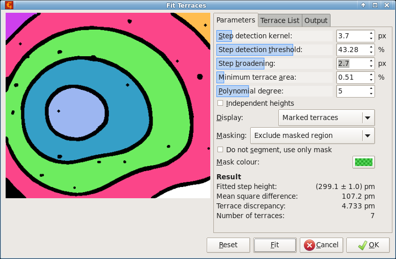
Terrace measurement dialogue screenshot showing marked terraces for an amphitheatre structure formed by atomic steps on silicon.

The lower part of tab Parameters shows an overview of the fitting results:

Tab Terraces contains a table detailing properties of individual terraces. Each row corresponds to one terrace. The columns are:

For relatively noisy data, discrepancies can be clearer indicators of correct fit than fit residua.

The resulting step height varies slightly with algorithm parameters. This dependence can be investigated using Survey by performing an automated scan over a range of polynomial degrees and/or step broadenings. All parameters not scanned in the survey are kept at values selected in the Parameters tab.

The survey is executed by pressing Execute and can take a while to finish. When it finishes a file dialogue will appear, allowing to choose the file where the resulting table should be saved.

[1] J. Garnæs, D. Nečas, L. Nielsen, M. Madsen, A. Torras-Rosell, G. Zeng, P. Klapetek, A. Yacoot, Algorithms for using silicon steps for scanning probe microscope evaluation. Metrologia 57 (2020) 064002, doi:10.1088/1681-7575/ab9ad3