Presentation modules do not modify the data, instead, they output their results into a separate layer displayed on top of the original data. The other data processing modules and tools will still operate on the underlying data. To remove a presentation, right-click on the data window, and select .
The → menu contains a few basic presentation operations:
Attaches another data field as a presentation to the current data. Note that this useful option can be particularly confusing while evaluating anything from the data as all the computed values are evaluated from the underlying data (not from the presentation, even if it looks like the data).
Removes presentation from the current data window. This is an alternative to the right-click data window menu.
Extracts presentation from the current data window to a new image in the same file. In this way one can get presentation data for further processing. Note, however, the extracted data have no absolute scale information as presentation often help to visualize certain features, but the produced values are hard or impossible to assign any physical meaning to. Hence the value range of the new image is always [0, 1].

→ →
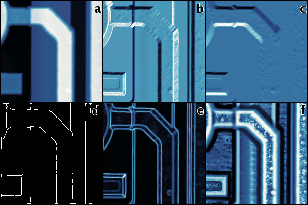
Simple and very useful way of seeing data as illuminated from some direction. The direction can be set by user. It is also possible to mix the shaded and original images for presentational purposes. Of course, the resulting image is meaningless from the physical point of view.


→ →
Sobel horizontal and vertical gradient filter and Prewitt horizontal and vertical gradient filter create similar images as shading, however, they output data as a result of convolution of data with relatively standardized kernel. Thus, they can be used for further presentation processing for example. The kernels for horizontal filters are listed below, vertical kernels differ only by reflection about main diagonal.

→ →
One is often interested in the visualization of the discontinuities present in the image, particularly in discontinuities in the value (zeroth order) and discontinuities in the derivative (first order). Although the methods of location of both are commonly referred to as “edge detection” methods, these are actually quite different, therefore we will refer to the former as to step detection and to the latter as to edge detection. Methods for the detection of more specific features, e.g. corners, are commonly used too, these methods usually are of order zero.
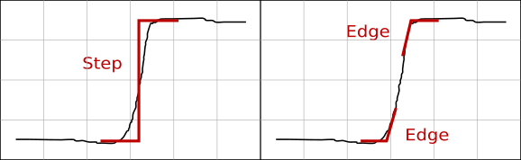
The order of a discontinuity detection method can be easily seen on its output as edge detection methods produce typical double edge lines at value discontinuities as is illustrated in the following figure. While the positions of the upper and lower edge in an ideal step coincide, real-world data tend to actually contain two distinct edges as is illustrated in the picture. In addition, finding two edges on a value step, even an ideally sharp one, is often an inherent feature of edge detection methods.
The following step and edge detection functions are available in Gwyddion (the later ones are somewhat experimental, on the other hand they usually give better results than the well-known algorithms):
- Canny
Canny edge detector is a well-known step detector that can be used to extract the image of sharp value discontinuities in the data as thin single-pixel lines.
- Laplacian of Gaussians
Laplacian presents a simple convolution with the following kernel (that is the limit of discrete Laplacian of Gaussians filter for σ → 0):
- Zero Crossing
Zero crossing step detection marks lines where the result of Laplacian of Gaussians filter changes sign, i.e. crosses zero. The FWHM (full width half maximum) of the Gaussians determines the level of details covered. Threshold enables to exclude sign changes with too small absolute value of the neighbour pixels, filtering out fine noise. Note, however, that for non-zero threshold the edge lines may become discontinuous.
- Step
A step detection algorithm providing a good resolution, i.e. sharp discontinuity lines, and a good dynamic range while being relatively insensitive to noise. The principle is quite simple: it visualizes the square root of the difference between the 2/3 and 1/3 quantiles of the data values in a circular neighbourhood of radius 2.5 pixels centred around the sample.
- Gaussian Step
Gaussian step is a tunable filter, with trade-off between fine tracing of the steps and resistance to noise. It has one parameter, width of the Gaussian (given as full width at half-maximum). Narrow filters produce fine lines, but also mark local defects. Wide filters distinguish better steps from other features, but the result is more blurred.
The filter works by convolving the image with kernels consisting of a Gaussian multiplied by sign function, rotated to cover different orientations. The results are then squared and summed together.
- RMS
This step detector visualizes areas with high local value variation. The root mean square of deviations from the mean value of a circular neighbourhood of radius 2.5 pixels centred around each sample is calculated and displayed.
- RMS Edge
This function essentially postprocesses RMS output with a filter similar to Laplacian to emphasize boundaries of areas with high local value variation. Despite the name it is still a step detector.
- Local Non-Linearity
An edge detector which visualizes areas that are locally very non-planar. It fits a plane through a circular neighbourhood of radius 2.5 pixels centred around each sample and then it calculates residual sum of squares of this fit reduced to plane slope, i.e. divided by 1 + bx2 + by2 where bx and by are the plane coefficients in x and y directions, respectively. The square root is then displayed.
- Inclination
Visualizes the angle ϑ of local plane inclination. Technically this function belongs among step detectors, however, the accentuation of steps in its output is not very strong and it is more intended for easy visual comparison of different slopes present in the image.
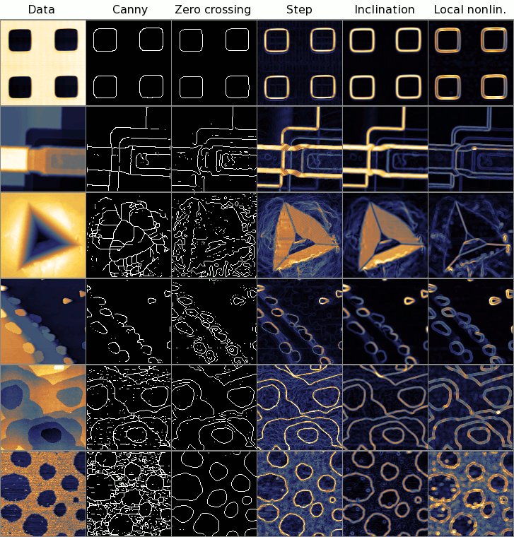
Comparison of step and edge detection methods on several interesting, or typical example data. Canny and Zero crossing are step detectors that produce one pixel wide edge lines, Step and Inclination are step detectors with continuous output, Local nonlinearity is an edge detector – the edge detection can be easily observed on the second and third row. Note zero crossing is tunable, it parameters were chosen to produce reasonable output in each example.
→ →
A method to visualize features in areas with low and high value variation at the same time. This is achieved by calculation of local value range, or variation, around each data sample and stretching it to equalize this variation over all data.
→ →
An alternative local contrast enhancement method. It is an equalising high-pass filter, somewhat complementary to the median filter. Each pixel value is transformed to its rank among all values from a certain neighbourhood. The neighbourhood radius can be specified as Kernel size.
The net effect is that all local maxima are equalised to the same maximum value, all local minima to the same minimum value, and values that are neither maxima nor minima are transformed to the range between based on their rank. Since the output of the filter with radius r can contain at most π(r + 1/2)2 different values (approximately), the filter also leads to value discretisation, especially for small kernel sizes.
→ →
The function renders an SEM image-like presentation from a topographical image using the simplest possible Monte Carlo method. For each surface pixel, a number of lines originating from this pixel are chosen with random directions and Gaussian length distribution. The standard deviation of the Gaussian distribution is controlled with the Integration radius parameters. If the other end of the line hits free space, the lightness in the origin pixel is increased. If it hits material, i.e. height value below the surface at the endpoint, the lightness is decreased. More precisely, this describes the Monte Carlo method. The number of lines can be controlled with the Quality parameter. Equivalently, the same intensity can be calculated by direct integration over all pixels within a circular neighbourhood. This corresponds to the Integration method.
Since even this simple computation can take a long time, it is useful to consider how its speed depends on the settings. The computation time for Integration depends only on the integration radius. The computation time for Monte Carlo, on the other hand, depends essentially only on Quality (there is also some dependence on the local topography).