Profiles taken in the fast scanning axis (usually x-axis) can be mutually shifted by some amount or have slightly different slopes. The basic line correction function Data Process → Correct Data → Align Rows deals with this type of discrepancy using several different correction algorithms:

Similarly as in the two-dimensional polynomial levelling, the background, i.e. values subtracted from individual rows can be extracted to another image. Or plotted in a graph since the value is the same for the entire row.

The line correction function support masking, allowing the exclusion of large features that could distract the correction algorithms. The masking options are offered only if a mask is present though. Note the Path level tools described below offers a different method of choosing the image parts important for alignment. It can be more convenient in some cases.

Line correction example: an image with defects (left), the row alignment dialogue previewing the median correction (centre), and extracted row background (right). Note the false colour scales are not the same in the three images.

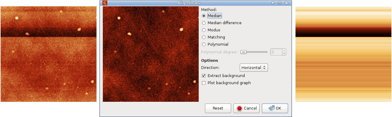
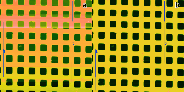
The Path Levelling tool can be used to correct the heights in an arbitrary subset of rows in complicated images.

First, one selects a number of straight lines on the data. The intersections of these lines with the rows then form a set of points in each row that is used for levelling. The rows are moved up or down to minimize the difference between the heights of the points of adjacent rows. Rows that are not intersected by any line are not moved (relatively to neighbouring rows).

Path Level example: (a) uncorrected data with steps that the automated method may fail to correct, two suitable levelling lines are selected; (b) the result of Path Level application with line width 5.

Function Step Line Correction attempts to deal with height jumps that may occur in the middle of a scan line. It tries to identify misaligned segments within the rows and correct the height of each such segment individually by subtracting its mean value. Therefore it is often able to correct data with discontinuities in the middle of a row.

This function is somewhat experimental and the exact way it works can be subject to further changes. Note that it still alignes all rows similarly to the Mean method in Align rows. See Block line correction for a method which attempts to only remove the jumps, preserving everything else.

Function Block Line Correction also attempts to correct jumps that may occur in the middle of a scan line. It also tries to change the image as little as possible, i.e. less than Step line correction which applies somewhat aggressive correction (and is thus generally more successful at removing the jumps as long as one does not mind the accompanying scan line flattening).

The block line correction identifies the sudden jumps, computes their heights and then shifts height in entire blocks of scan lines between them. That is where the name “block” comes from. In regions where no sudden jump occured mutual the height relations bewtween scan lines are perfectly preserved.

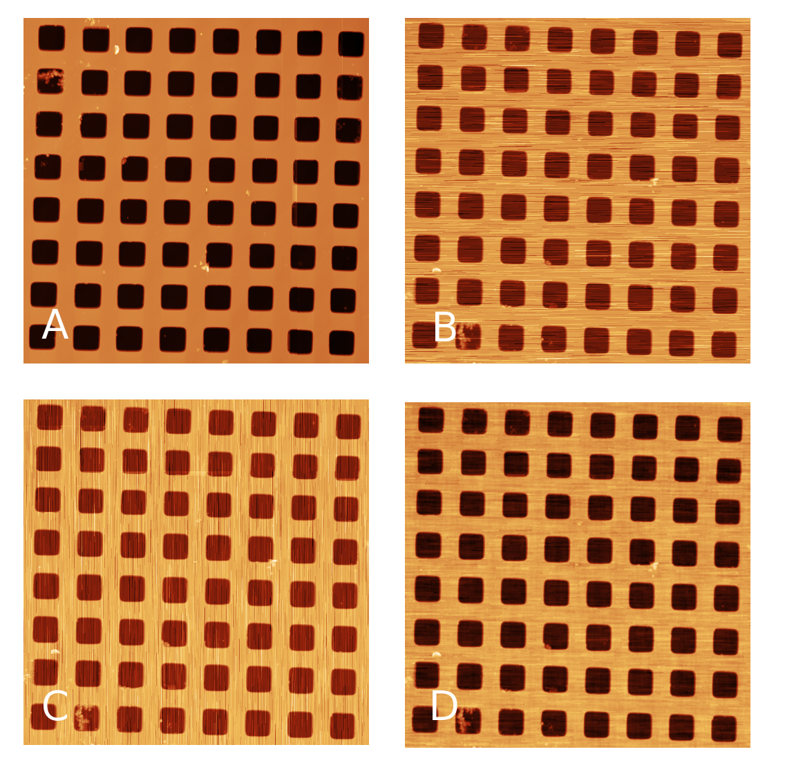
Since entire blocks are shifted the direction of scanning is important in determining which pixels from a contiguous block. It has to be selected as Scanning direction. The directions are labelled as for scanning from top to bottom in the slow axis. For scanning from the bottom upwards the meaning is reversed. If the functions seems unable to notice obvious jumps check that the direction is correct.

Step artefacts examples for top-to-bottom scanning in the slow axis. Left: left-to-right. Right: right-to-left.

Threshold determines the sensitivity, in other words how large jumps are considered discontinuities. It is given as a multiple of the root mean square of all differences between two vertical neighbour pixels. By selecting Marked discontinuities in Display one can get an overview of all locations where the height difference exceeds given threshold. The option Marked block boundaries is probably more useful as is shows where a discontinuity spans the entire image width and is, therefore, considered a boundary between two blocks. The number of total detected jumps is displayed below Threshold.

Taking mean or median rows from the entire image using Row/Column Statistics tool can provide clean profiles from images formed by repeated scanning of the same feature. This is sometimes done with slow scanning axis disabled entirely, other times with scanning enabled but with much reduced range in the slow axis. If defects are present they should be excluded by masking. When both forward and backward scans are available, comparing them can help determining which parts of the profiles are good and which contain defects.

The Mean Good Profile function simplifies this in a couple of common situations:

In both modes either the profile graph is shown, or the image with corresponding mask of excluded pixels. The module also shows the variation, i.e. the integral of the absolute value of the derivative. Large variation means more noisy or jagged profile. Hence, lower values usually correspond to better profiles.

Function Mark Inverted Rows finds scan lines with vertically inverted features and marks them with a mask. Line inversion is an artefact which occasionally occurs for instance in Magnetic Force Microscopy. Since the line is generally only inverted very approximately, value inversion would be a poor correction and one should usually use Laplace's interpolation for correction.

Data Process → Correct Data → Mark Scars

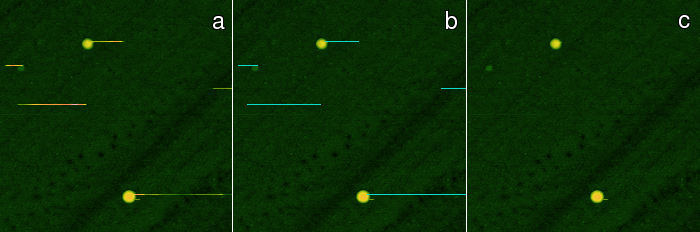
Similarly, the Mark Scars module can create a mask of the points treated as scars. Unlike Remove Scars which directly interpolates the located defects, this module lets you interactively set several parameters which can fine-tune the scar selection process:

After clicking Ok the new scar mask will be applied to the image. Other modules or tools can then be run to edit this data.

Scars marking and removal example: (a) original data with defects, (b) data with marked defects, (c) corrected data.

Data Process → Correct Data → Remove Scars

Scars (or stripes, strokes) are parts of the image that are corrupted by a very common scanning error: local fault of the closed loop. Line defects are usually parallel to the fast scanning axis in the image. This function will automatically find and remove these scars, using neighbourhood lines to “fill-in” the gaps. The method is run with the last settings used in Mark Scars.

Data Process → Multidata → XY denoise

The function denoises and image on the basis of two measurements of the same area – one performed in x direction and one in y direction (and rotated back to be aligned the same way as the x-direction one). It is based on work of E. Anguiano and M. Aguilar (see [1]).

The denoising works by performing the Fourier transform of both images, combining the information them in the frequency space, and then using backward Fourier transform in order to get the denoised image. It is useful namely for the removal of large scars and fast scanning axis stripes.

The images do not appear symmetrically in the procedure. By using option Average denoising directions one can apply it in both ways and average the results.

XY denoise procedure simulation: A) original data, B) simulated measurement in x axis, C) simulated measurement in y axis, D) denoised image.

[1] E. Anguiano and M. Aguilar: A cross-measurement procedure (CMP) for near noise-free imaging in scanning microscopes. Ultramicroscopy, 76 (1999) 47 doi:10.1016/S0304-3991(98)00074-6