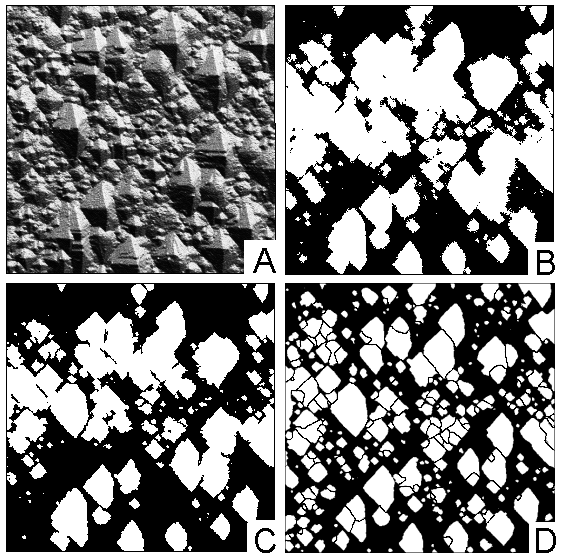
There are several grain-related algorithms implemented in Gwyddion. First of all, simple thresholding algorithms can be used (height, slope or curvature thresholding). These procedures can be very efficient namely within particle analysis (to mark particles located on flat surface).

→ →
Thresholding is the basic grain marking method. Height, slope and curvature thresholding is implemented within this module. The results of each individual thresholding methods can be merged together using logical operators.

→ →
The automated Otsu's thresholding method classifies the data values into two classes, minimising the intra-class variances within both. It is most suitable for images that contain two relatively well defined value levels.

→ →
Another grain marking function is based on edge detection (local curvature). The image is processed with a difference-of-Gaussians filter of a given size and thresholding is then performed on this filtered image instead of the original.

→ →
Grains that touch image edges can be removed using this function. It is useful if such grains are considered incomplete and must be excluded from analysis. Several other other functions that may be useful for modification of grain shapes after marking are performed by the Mask Editor tool.

→ →
For more complicated data structures the effectiveness of thresholding algorithms can be very poor. For these data a watershed algorithm can be used more effectively for grain or particle marking.
The watershed algorithm is usually employed for local minima determination and image segmentation in image processing. As the problem of determining the grain positions can be understood as the problem of finding local extremes on the surface this algorithm can be used also for purposes of grain segmentation or marking. For convenience in the following we will treat the data inverted in the z direction while describing the algorithm (i.e. the grain tops are forming local minima in the following text). We applied two stages of the grain analysis (see [1]):
- Grain location phase: At each point of the inverted surface the virtual water drop was placed (amount of water is controlled by parameter Drop size). In the case that the drop was not already in a local minimum it followed the steepest descent path to minimize its potential energy. As soon as the drop reached any local minimum it stopped here and rested on the surface. In this way it filled the local minimum partially by its volume (see figure below and its caption). This process was repeated several times (parameter Number of steps). As the result a system of lakes of different sizes filling the inverted surface depressions was obtained. Then the area of each of the lakes was evaluated and the smallest lakes are removed under assumption that they were formed in the local minima originated by noise (all lakes smaller than parameter Threshold are removed). The larger lakes were used to identify the positions of the grains for segmentation in the next step. In this way the noise in the AFM data was eliminated. As a result
-
Segmentation phase: The grains found in the step 1 were marked (each one by a different
number). The water drops continued in falling to the surface and
filling the local minima (amount of water is controlled by parameter Drop size).
Total number of steps of splashing a drop at every surface position is controlled by parameter Number of steps.
As the grains were already identified and
marked after the first step, the next five situations could happen as
soon as the drop reached a local minimum.
- The drop reached the place previously marked as a concrete grain. In this case the drop was merged with the grain, i. e. it was marked as a part of the same grain.
- The drop reached the place where no grain was found but a concrete grain was found in the closest neighbourhood of the drop. In this case the drop was merged with the grain again.
- The drop reached the place where no grain was found and no grain was found even in the closest neighbourhood of the drop. In that case the drop was not marked at all.
- The drop reached the place where no grain was found but more than one concrete grain was found in the closest neighbourhood (e. g. two different grains were found in the neighbourhood). In this case the drop was marked as the grain boundary.
- The drop reached the place marked as grain boundary. In this case the drop was marked as the grain boundary too.
In this way we can identify the grain positions and then determine the volume occupied by each grain separately. If features of interest are valleys rather than grains (hills), parameter Invert height can be used.
→ →
This function a different approach based on a watershed algorithm, in this case the classical Vincent algorithm for watershed in digital spaces [2], which is applied to a preprocessed image. Generally, the result is an image fully segmented to motifs, each pixel belonging to one or separating two of them. By default, the algorithm marks valleys. To mark upward grains, which is more common in AFM, use the option Invert height.
The preprocessing has the following parameters:
- Gaussian smoothing
Dispersion of Gaussian smoothing filter applied to the data. A zero value means no smoothing.
- Add gradient
Relative weight of local gradient added to the data. Large values mean areas with large local slope tend to become grain boundaries.
- Add curvature
Relative weight of local gradient added to the data. Large values mean locally concave areas with tend to become grain boundaries.
- Barrier level
Relative height level above which pixels are never assigned to any grain. If not 100%, this creates an exception to the full-segmentation property.
- Prefill level
Relative height level up to which the surface is prefilled, obliterating any details at the bottoms of deep valleys.
- Prefill from minima
Relative height level up to which the surface is prefilled from each local minimum, obliterating any details at the bottoms of valleys.
→ →
To transfer segmentation from one image to another one with similar features, or from small chunk to complete large image, the logistic regression module can be used. It has two modes of operation, in training phase it requires the mask of grains to be present on the image, and train logistic regression for this mask. When the regression is trained, one can use it for the new images. In both modes it generates a feature vector from the current image, applying a number of filters to it. The available features include:
- Gaussian blur
Gaussian filters with the length of 2, 4, 8 and so on. The number of gaussians can be selected by the user with Number of Gaussians
- Sobel derivatives
Sobel first derivative filters for X and Y directions.
- Laplacian
Laplacian sum of second deriatives operator.
- Hessian
three elements of Hessian matrix of second derivatives, one for each of X- and Y-directions and one mixed.
All derivative filters if selected are applied to original image as well as to each of Gaussian-filtered if they present. Each feature layer is computed with the convolution operator and than normalized.
Regularization parameter allows to regularize logistic regression, larger values means that parameters are more restricted from having very large values.
Note, that you need to have a mask on image for training, or the training will give zero results. The training phase can be very slow, especially for large images and large set of features selected. The training results are saved between the invocation, so they can be applied to other images. If the set of features is modified, one need to train logistic regression from the scratch.
Grain properties can be studied using several functions. The simplest of them is Grain Summary.
→ →
This function calculates the total number of marked grains, their total projected area, both as an absolute value and as a fraction of total data field area, total grain volumes, total length of grain boundaries and the mean area and equivalent square size of one grain. The mean size is calculated by averaging the equivalent square sides so its square is not, in general, equal to the mean area.
Overall characteristics of the marked area can be also obtained with Statistical Quantities tool when its Use mask option is switched on. By inverting the mask the same information can be obtained also for the non-grain area.
→ →
The grain statistics function displays the mean, median, standard deviation (rms) and inter-quartile range for all available grain quantities in one table.

→ →
Grain Distributions is the most powerful and complex tool. It has two basic modes of operation: graph plotting and raw data export. In graph plotting mode selected characteristics of individual grains are calculated, gathered and summary graphs showing their distributions are plotted.
Raw data export is useful for experts who need for example to correlate properties of individual grains. In this mode selected grain characteristics are calculated and dumped to a text file table where each row corresponds to one grain and columns correspond to requested quantities. The order of the columns is the same as the relative order of the quantities in the dialogue; all values are written in base SI units, as is usual in Gwyddion.

→ →
Grain correlation plots a graph of one selected graph quantity as the function of another grain quantity, visualizing correlations between them.

The grain measurement tool is the interactive method to obtain the same information about individual grains as Grain Distributions in raw mode. After selecting a grain on the data window with mouse, all the available quantities are displayed in the tool window.
Beside physical characteristics this tool also displays the grain number. Grain numbers corresponds to row numbers (counting from 1) in files exported by Grain Distributions.
Grain Distributions and Grain measurement tool can calculate the following grain properties:
- Value-related properties
- Minimum, the minimum value (height) occurring inside the grain.
- Maximum, the maximum value (height) occurring inside the grain.
- Mean, the mean of all values occurring inside the grain, that is the mean grain height.
- Median the median of all values occurring inside the grain, that is the median grain height.
- RMS the standard deviation of all values occurring inside the grain.
- Minimum on boundary, the minimum value (height) occurring on the inner grain boundary. This means within the set of pixels that lie inside the grain but at least one of their neighbours lies outside.
- Maximum on boundary, the maximum value (height) occurring on the inner grain boundary, defined similarly to the minimum.
- Area-related properties
- Projected area, the projected (flat) area of the grain.
- Equivalent square side, the side of the square with the same projected area as the grain.
- Equivalent disc radius, the radius of the disc with the same projected area as the grain.
- Surface area, the surface area of the grain, see statistical quantities section for description of the surface area estimation method.
- Area of convex hull, the projected area of grain convex hull. The convex hull area is slightly larger than the grain area even for grains that appear to be fairly convex due to pixelisation of the mask. The only grains with exactly the same area as their convex hulls are perfectly rectangular grains.
- Boundary-related properties
- Projected boundary length, the length of the grain boundary projected to the horizontal plane (that is not taken on the real three-dimensional surface). The method of boundary length estimation is described below.
- Minimum bounding size, the minimum dimension of the grain in the horizontal plane. It can be visualized as the minimum width of a gap in the horizontal plane the grain could pass through.
- Minimum bounding direction, the direction of the gap from the previous item. If the grain exhibits a symmetry that makes several directions to qualify, an arbitrary direction is chosen.
- Maximum bounding size, the maximum dimension of the grain in the horizontal plane. It can be visualized as the maximum width of a gap in the horizontal plane the grain could fill up.
- Maximum bounding direction, the direction of the gap from the previous item. If the grain exhibits a symmetry that makes several directions to qualify, an arbitrary direction is chosen.
- Maximum inscribed disc radius, the radius of maximum disc that fits inside the grain. The entire full disc must fit, not just its boundary circle, which matters for grains with voids within. You can use Mask Editor tool to fill voids in grains to get rid of voids.
- Maximum inscribed disc centre x position, the horizontal coordinate of centre of the maximum inscribed disc. More precisely, of one such disc if it is not unique.
- Maximum inscribed disc centre y position, the vertical coordinate of centre of the maximum inscribed disc. More precisely, of one such disc if it is not unique but of the same as in the previous item.
- Minimum circumcircle radius, the radius of minimum circle that contains the grain.
- Minimum circumcircle centre x position, the horizontal coordinate of centre of the minimum circumcircle.
- Minimum circumcircle centre y position, the vertical coordinate of centre of the minimum circumcircle.
- Mean radius, the mean distance from grain centre of mass to its boundary. This quantity is mostly meaningful only for convex or nearly-convex grains.
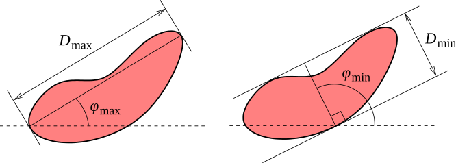
- Minimum Martin diameter, the minimum length of a median line through the grain.
- Direction of minimum Martin diameter, the direction of the line from the previous item. If the grain exhibits a symmetry that makes several directions to qualify, an arbitrary direction is chosen.
- Maximum Martin diameter, the maximum length of a median line through the grain.
- Direction of maximum Martin diameter, the direction of the line from the previous item. If the grain exhibits a symmetry that makes several directions to qualify, an arbitrary direction is chosen.
- Volume-related properties
- Zero basis, the volume between grain surface and the plane z = 0. Values below zero form negative volumes. The zero level must be set to a reasonable value (often Fix Zero is sufficient) for the results to make sense, which is also the advantage of this method: one can use basis plane of his choice.
- Grain minimum basis, the volume between grain surface and the plane z = zmin, where zmin is the minimum value (height) occuring in the grain. This method accounts for grain surrounding but it typically underestimates the volume, especially for small grains.
- Laplacian backround basis, the volume between grain surface and the basis surface formed by laplacian interpolation of surrounding values. In other words, this is the volume that would disappear after using Interpolate Data Under Mask or Grain Remover tool with Laplacian interpolation on the grain. This is the most sophisticated method, on the other hand it is the hardest to develop intuition for.
- Position-related properties
- Centre x position, the horizontal coordinate of the grain centre. Since the grain area is defined as the area covered by the corresponding mask pixels, the centre of a single-pixel grain has half-integer coordinates, not integer ones. Data field origin offset (if any) is taken into account.
- Centre y position, the vertical coordinate of the grain centre. See above for the interpretation.
- Slope-related properties
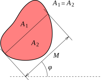
- Inclination θ, the deviation of the normal to the mean plane from the z-axis, see inclinations for details.
- Inclination φ, the azimuth of the slope, as defined in inclinations.
- Curvature-related properties
- Curvature centre x, the horizontal position of the centre of the quadratic surface fitted to the grain surface.
- Curvature centre y, the vertical position of the centre of the quadratic surface fitted to the grain surface.
- Curvature centre z, the value at the centre of the quadratic surface fitted to the grain surface. Note this is the value at the fitted surface, not at the real grain surface.
- Curvature 1, the smaller curvature (i.e. the inverse of the curvature radius) at the centre.
- Curvature 2, the larger curvature (i.e. the inverse of the curvature radius) at the centre.
- Curvature angle 1, the direction corresponding to Curvature 1.
- Curvature angle 2, the direction corresponding to Curvature 2.
- Moment-related properties
- Major semiaxis of equivalent ellipse, the length of the major semiaxis of an ellipse which has the same second order moments in the horizontal plane.
- Minor semiaxis of equivalent ellipse, the length of the minor semiaxis of an ellipse which has the same second order moments in the horizontal plane.
- Orientation of equivalent ellipse, the direction of the major semiaxis of an ellipse which has the same second order moments in the horizontal plane. For a circular grain, the angle is set to zero by definition.
The grain boundary length is estimated by summing estimated contributions of each four-pixel configuration on the boundary. The contributions are displayed on the following figure for each type of configuration, where hx and hy are pixel dimension along corresponding axes and h is the length of the pixel diagonal:
The contributions correspond one-to-one to lengths of segments of the boundary of a polygon approximating the grain shape. The construction of the equivalent polygonal shape can also be seen in the figure.
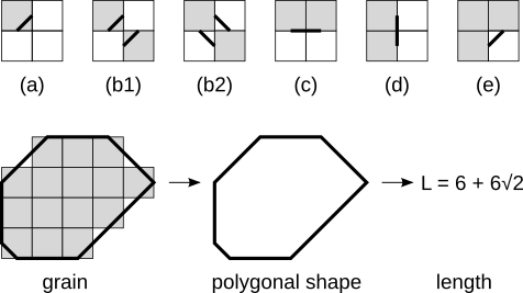
Contributions of pixel configurations to the estimated boundary length (top). Grey squares represent pixels inside the grain, white squares represent outside pixels. The estimated contribution of each configuration is: (a) h/2, (b1), (b2) h, (c) hy, (d) hx, (e) h/2. Cases (b1) and (b2) differ only in the visualization of the polygonal shape segments, the estimated boundary lengths are identical. The bottom part of the figure illustrates how the segments join to form the polygon.
The grain volume is, after subtracting the basis, estimated as the volume of exactly the same body whose upper surface is used for surface area calculation. Note for the volume between vertices this is equivalent to the classic two-dimensional trapezoid integration method. However, we calculate the volume under a mask centred on vertices, therefore their contribution to the integral is distributed differently as shown in the following figure.
Curvature-related properties of individual grains are calculated identically to the global curvature calculated by Curvature. See its description for some discussion.
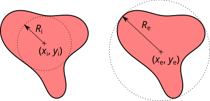
Inscribed discs and circumcircles of grains can be visualized using → → and → → . These functions create circular selections representing the corresponding disc or circle for each grain that can be subsequently displayed using Selection Manager tool.
The Martin's diameter is the length of the unique line through the grain in given direction which which divides the grain area into two equal parts (median line). This quantity is mostly useful for grains that are still relatively close to convex. For reference we should note that if the grain is highly non-convex and the median line intersects the grain several times, Gwyddion sums the lengths of the segments actually lying inside the grain (the other option would be to simply take the distance between the first and last intersection).

Marked grains can be filtered by thresholding by any of the available grain quantities using → → menu choice. The module can be used for basic operations, such as removal of tiny grains using a pixel area threshold, as well as complex filtering using logical expressions involving several grain quantities.
The filter retains grains that satisfy the condition specified as
Keep grains satisfying and removes all other
grains. The condition is expressed as a logical expression of one to
three individual thresholding conditions, denoted A,
B and C. The simplest expression
is just A, stating that quantity
A must lie within given thresholds.
Each condition consits of lower and upper thresholds for one grain quantity, for instance pixel area or minimum value. The values must lie within the interval [lower,upper] to satisfy the condition and thus retain the grains. Note it is possible to choose the lower threshold larger than the upper threshold. In this case the condition is inverted, i.e. the grain is retained if the value lies outside [upper,lower].
Individual grain quantities are assigned to A,
B and C by selecting the
quantity in the list and clicking on the corresponding button in
Set selected as. The currently selected set of
quantities is displayed in the
Condition A,
Condition B and
Condition C headers.
→ →
When images with marked grains are further processed in other software, it can be useful to clearly identify which region corresponds has which grain number assigned in Gwyddion. This function creates an image where each pixel contains the corresponding grain number. Hence, even though the data are still floating point numbers all the values are in fact integers.
Grains can be aligned vertically using → → . This function vertically shifts each grain to make a certain height-related quantity of all grains equal. Typically, the grain minimum values are aligned but other choices are possible.
Data between grains are also vertically shifted. The shifts are interpolated from the grain shifts using the Laplace equation, leading to a smooth transition of the shifts between the grains (though with no regard to other possible surface features).
[1] P. Klapetek, I. Ohlídal, D. Franta, A. Montaigne-Ramil, A. Bonanni, D. Stifter, H. Sitter: Atomic force microscopy characterization of ZnTe epitaxial films. Acta Physica Slovaca 53 (2003) 223–230, doi:10.1143/JJAP.42.4706
[2] Luc Vincent and Pierre Soille: Watersheds in digital spaces: an efficient algorithm based on immersion simulations. IEEE Transactions on Pattern Analysis and Machine Intelligence, 13 (1991) 583–598, doi:10.1109/34.87344