In MFM measurements we collect information about stray field distribution above sample, typically in one layer in fixed height above sample during one measurement. Together with this signal, we collect also topography, similarily to all the other SPM techniques.
The functions specific to MFM can be found in the → → . The individual modules and data processing algorithms discussed in the following paragraphs can be split into several categories:
- utility functions, such as conversion of different quantities to force gradient,
- modules for simulation of the MFM response on different samples (e.g. perpendicular media or a thin film stripe with electrical current),
- probe analysis modules based on use of known samples, and
- sets of functions for handling multiple channel data, e.g. data measured with opposite tip magnetisation.
The last category includes general functions such as data arithmetic which can add subtract images and generally combine them using arithmetic expressions or mutual crop which cuts images to the common sub-region (and is often a prerequsite for multi-data operations).
Addition and subtraction of measurements performed with two different probe magnetisation directions was proposed as the means of potential improvement of the process of splitting the magnetic and other contributions [Cambel11]. If measurements with different current direction are also available, we have four possible variants of how the electrostatic and magnetic forces are mutually oriented. All four can be comined to using data arithmetic to supress the noise in the data
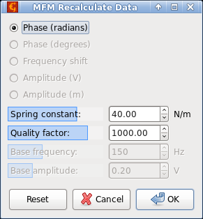
Function performs conversion of various measured quantities to force gradient. The input image must correspond to one of the quantities for which the conversion is implemented, phase, frequency shift or amplitude (in Volts or metres). The type of input data is automatically determined and indicated by the input quantity choice in the upper part.
The conversion requires entering instrumental parameters, which differ depending on the input data and may include the sprint constant, quality factor or base amplitude.
Several modules, differing by the algorithm used, simulate the stray field distribution in a plane above sample surface. None of them works with a general medium — e.g. using Poisson equation to solve the magnetic field distribution from the samle volume magnetisation — as this seems to be too computationally demanding for a general package like Gwyddion (at least for now). The modules are set up to simulate a few typical cases described in literature, where there are enough assumptions about sample magnetisation to make the stray field calculable by simple methods.
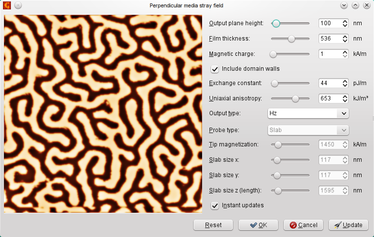
The module for handling perpendicular media is based on works of H. Hug [Hug98] and S. Vock [Vock11][Vock14]. The field distribution is calculated on the basis of known magnetisation distribution in a layer; in the z direction the magnetisation is constant for each position in the layer and changes only when we go in lateral directions. Initially, magnetisation is described as binary image (up/down magnetisation, defined by mask) and domain walls of given thickness can be added to it. The calculation is then done in Fourier space. Apart of the magnetic field distribution also results of using simple analytically known probe transfer functions can be provided (point charge, bar), and numerical derivatives of the resulting forces can be computed.
Assuming the surface charge distribution +σ(x, y) at the top surface of the medium and opposite charge −σ(x, y) at the bottom surface we can use Fourier analysis to get the field distribution. First we convert the surface charges to the Fourier space:
Optionally we can even assume that in between of the domains there are Bloch walls of some width δw, convolving σ(x, y) prior to the calculation with blurring operator
where the wall width can be expressed via exchange stiffness constant A and uniaxial anisotropy constant Ku as
Then we can calculate the Fourier components of the stray field in height z, generated from top surface and bottom surface of film of thickness d as
Via inverse Fourier transform we can then get the magnetic stray field above the sample:
While still staying in the Fourier space, we can also calculate the force acting on a simple bar probe of cross-section bx × by, length L and magnetisation Mt, by multiplying the stray field components length AHzz, d via the analytical force transfer function:
Since Gwyddion is not just able to handle measured data, but also to synthetise many different artificial surfaces, there are many ways how to play with the perpendicular media module, creating various fields on more or less realistic samples. The following figure shows few examples of such simulated masks and resulting data.
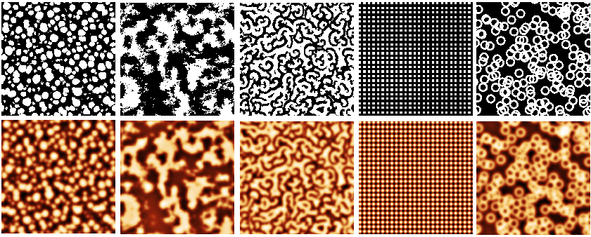
Result of data synthetic modules used for MFM perpendicular media simulation: columnar film, fractal roughness, Ising model domains, grating, doughnuts.
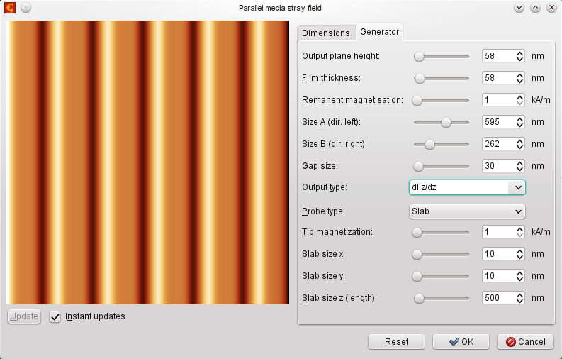
For parallell media the range of potential calculations is much smaller — based on an analytical model the field above left and right direction oriented stripes (similar to a hard-disc) can be computed. This is based on [Rugar90], giving the following equations for individual transitions
where Mr, is the remanent magnetization of the magnetic layer, z the tip-sample separation, a is the transition area width, and d the layer thickness.
The stripes do not have to be of equal size. As a result, field intensities in x and z axes can be plotted, or the force in z based on known probe transfer functions (the same as for the perpendicular media) can be computed. Its derivatives can be computed as well (numerically).
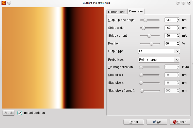
Similarily, analytical expressions can be used to simulate the current above a thin line with a electrical current passing through it. The current line module can be used for this, which is based on the equation given by [Saida03]:
for a stripe of width w in which the current I is flowing.
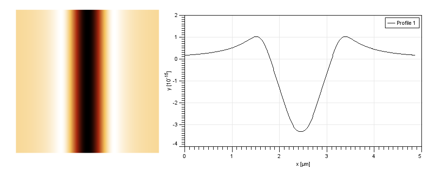
As all the simulation modules can be used also to add the result to existing data, by calling module multiple times we can also simulate a planar coil (or, more precisely, two lines with opposite directions of the current). This is demonstrated in the following figures.
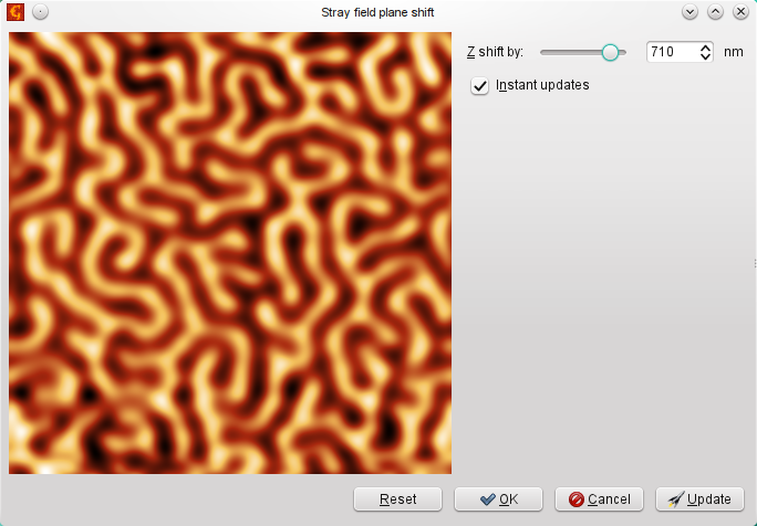
The algorithms for stray field calculation via Fourier transform can be also used to shift the field from one layer height to another. This works if we move further from the sample (blurring the data), but it does not work much when getting closer to the sample (the calculation diverges). Based on [Hug98] the procedure is as follows:
- The field Hz(r) is processed by Fourier transform to get its spectral representation AHz(k),
- Spectral components are multiplied by the factor exp(kd) where d is the distance between the two planes (positive or negative),
- Inverse Fourier transform is used to get back the field values in real space.
One can play with this algorithm in the field shift module as illustrated in the following figure.
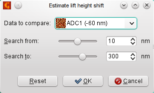
The same approach can be used for reverse operation — estmating the height difference between two data sets. Here a simple brute force search technique is used to find the shift in z direction that leads to best match between the two MFM responses. The user interface is shown in Fig. 8. Potential application is in searching for the real lift height difference instead of the reported one, however there are still potential caveats in real data if there are parasitic interactions.
Several ways have been proposed how to handle the issue of resolution of MFM probes. It is possible to analyse profiles across the perpendicular sample or utilise the power spectrum for probe resolution, e.g. by attempting to find where the power spectrum vanishes to noise level. See Transfer Function Guess for the transfer function estimation method currently implemented in Gwyddion. This technique is not, in fact, specific to MFM and can be used universally for transfer function TF (or point spread function, PSF) estimation in any SPM regime, provided that the ideal sample response can be recorded or simulated. The mathematical and algorithmic details on how the magnetic data are treated in the transfer function modules can be found in Ref. Nečas19.
To illustrate the whole procedure of obtaining quantitative MFM results we provide here an example of the transform function estimation on a known sample and data processing of data obtained on an unknown sample, based on this transfer function.
The starting point is to use the data measured on a known sample. Here a multilayer sample manufactured by IFW Dresden is used, for which the stray field above sample can be computed on basis of the known domains distribution and known sample properties. Together with this, the “unknown” test sample data, provided by National Physical Laboratory are in the same input file available for download.
To go step by step and get the same results as provided in the processed file, the following procedure has to be done:
- Convert calibration sample MFM phase data to MFM force gradient using Recalculate to Force Gradient with k 3.3 N/m and Q factor 226.
- Add mask at 50% of the value using thresholding.
- Calculate the effective magnetic charge using Perpendicular Media Stray field with 130 nm film thickness, 500 kA/m magnetic charge, 12 pJ/m exchange constant, 400 kJ/m³ uniaxial anisotropy, 0 deg cantilever angle and output Meff.
- Calculate the TTF using Transfer Function Guess with Wiener filter method, 65×65 TTF size and Welch window.
- Convert MFM phase data of the test sample to MFM force gradient using Recalculate to Force Gradient with k 3.3 N/m and Q factor 226.
- Scale the TTF to the pixel size of the test sample.
- Use Dimensions and Units to match exactly the pixel size of the test sample measurements.
- Deconvolve the cropped TTF from MFM force gradient on test sample using Deconvolve, using the maxium of L-curve curvature for obtaining best sigma.
- Divide the resulting effective magnetic charge by 2 to get the stray field Hz using Arithmetic.
[Hug98] H. J. Hug, B. Stiefel, P. J. A. van Schendel, A. Moser, R. Hofer, S. Martin, H.-J. Gutherodt, S. Porthun, L. Abelmann, J. C. Lodder, G. Bochi and R. C. O’Handley: J. Appl. Phys. (1999) Vol. 83, No. 11
[Vock11] S. Vock, Z Sasvari, C. Bran, F. Rhein, U. Wolff, N. S. Kiselev, A. N. Bogdanov, L. Schiltz, O. Hellwig and V. Neu: IEEE Trans. on Magnetics, 47 (2011) 2352
[Vock14] S. Vock, C. hengst, M. Wolf, K. Tschulik, M. Uhlemann, Z. Sasvari, D. Makarov, O. G. Schmidt, L Schultz and V. Neu: Appl. Phys. Lett 105 (2014) 172409
[Rugar90] D. Rugar, H. J. Mamin, P. Guethner, S. E. Lambert, J. E. Stern et al.: J. Appl. Phys. 68 (1990) 1169
[Saida03] D. Saida, T. Takahashi: Jpn. J. Appl. Phys. 42 (2003) Pt. 1, No. 7B
[Cambel11] V. Cambel, D. Gregusova, P. Elias, J. Fedor, I. Kostic, J. Manka, P. Ballo: Journal of Electrical Engineering, 62 (2011) 37–43
[Necas19] D. Nečas, P. Klapetek, V. Neu, M. Havlíček, R. Puttock, O. Kazakova, X. Hu, L. Zajíčková, Scientific Report, 9 (2019) 3880