Several Gwyddion functions do convolutions and deconvolutions of some sort. A subtle point which is occasionaly a source of confusion is the difference between continuous and discrete operations. When images f and g are physical quantities, i.e. fields sampled in space, their convolution h
is again a physical field. Its physical dimension (units) is
For images dim(A) has the dimension of image area, i.e. usually square metres.
When the integral is realized using a discrete Riemann sum
the area appears as the area of one pixel ΔA. This is how all Gwyddion convolution, deconvolution and transfer function operations work by default, i.e. with the Normalize as integral option enabled.
In digital image processing physical units are sometimes ignored and convolution understood as simple discrete convolution of images
It is possible to obtain this behaviour by disabling the option Normalize as integral in a particular function. You should be aware the result of the operation is then no longer a physical quantity sampled in space (it depends on pixel size) and the units are different. The only function which works this way by default is Convolution Filter, where one of the operands is given as a small matrix of unitless numbers.

→ →
Convolution of two images can be performed using Convolve (see Convolution Filter for convolution with a small kernel, entered numerically). The module has only a few options:
- Convolution kernel
- The smaller image to convolve the larger image with, for instance a tip transfer function image. The dimensions of one pixel in both images must correspond.
- Exterior type
- What values should be assumed for pixels outside the image (as in Extend).
- Output size
- The size of the resulting image with respect to which pixels entered the calculation. Crop to interior cuts the image to consists only of pixels that are sufficiently far from the boundary that the exterior does not matter. Keep size creates an image with the same as the input image. Finally, Extend to convolved means the resulting image will be extended on each side by half the kernel size.

→ →
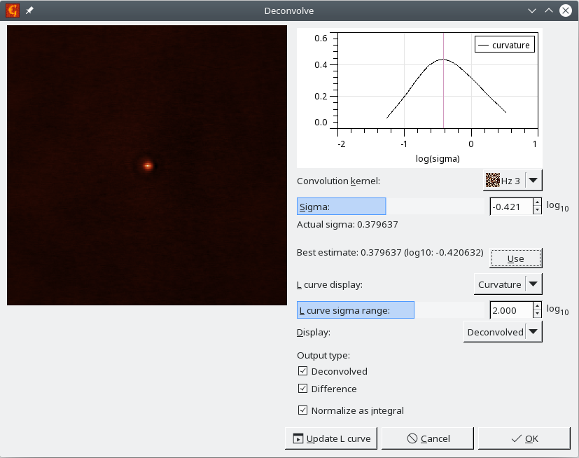
A simple regularized deconvolution of two images can be performed using Deconvolve. L-curve method can be used to search for the optimum regularization parameter, however its applicability highly depends on the data. The module has the following options:
- Convolution kernel
- The kernel to be deconvolved from the current image.
- Sigma
- Regularization parameter.
- L-curve display
- The data to be shown in the optional L-curve plot, when this is computed. The L-curve consist of two data sources: difference between the result convolved with the kernel and the original data and norm of the result. These two are plotted in a log-log graph providing a L-curve, but their dependences on the regularization parameters can be plotted also individually. The curvature of the resulting curve vs. regularization parameter gives the usual criterion for the best regularization parameters, seeking for the curve maximum.
- L-curve sigma range
- Range of the regularization parameter to be used in the L-curve calculation. This is, similarly to the regularization parameter, logarithmic, so it can span very large range, not necessarily suitable for the particular data set.
Output type Deconvolved produces the deconvolved image; Difference calculates the difference between reconvolved image and the input.
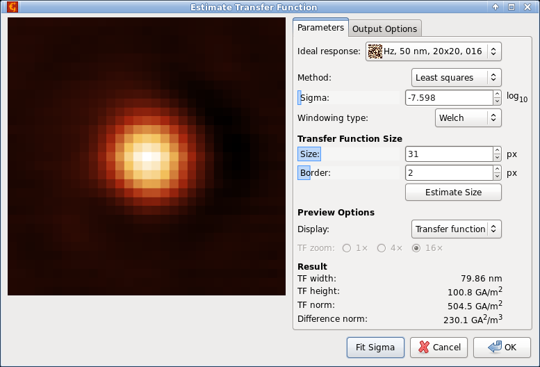
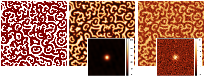
The probe transfer function (or point spread function) can be estimated from measured data, even noisy, when the corresponding ideally sharp signal is available. Gwyddion currently implements a few relatively simple methods.
→ → . The user interface of the module is and a typical performance on simulated noisy data is shown in the following figures.
The sharp signal is selected as Ideal response. It must have the same dimensions as the image. In contrast to the general Deconvolve module this module is optimized for the statistical properties of the transfer functions. There are currently three available deconvolution methods:
- Regularised filter
Simple frequency-space filter with constant regularisation term. It produces transfer function image of the same size as the input images. Option TF zoom can be used to display zoomed central part of the image.
- Least squares
The transfer function is found by solving the least squares problem corresponding to the deconvolution. The size of transfer function can be chosen arbitrarily. Usually it is much smaller than the input images.
Parameter Size controls the transfer function image size. If Border is nonzero, the transfer function image is enlarged by this value before solving the least squares problem and then the border is cut. A small border of 2 or 3 often improves the result because errors tend to accumulate in the edge pixels. Both sizes can be estimated automatically using .
- Wiener filter
Pseudo-Wiener filter assuming the spectral density of the output can be estimated by the spectral density of the input image. It is again a frequency-domain filter, producing transfer function image of the same size as the input images. Option TF zoom can be used to display zoomed central part of the image.
Two important parameters influence the result. The dimensionless regularisation parameter σ, which is used in all the methods, but is not directly comparable between them. It can be chosen manually. Since suitable values can differ by several orders of magnitude, it is presented as base-10 logarithm. However, the module can find a suitable value also automatically when is pressed.
determines the windowing function applied to both input images before deconvolution. Unless the input data are periodic, windowing is a necessity to avoid cross-like artefacts in the transfer function. The default Welch window is usually a good choice.
A few characteristics of the transfer function are immediately displayed in the bottom part of the dialogue as Result:
- TF width
- Width, calculated as square root of dispersion when the transfer function is taken as a distribution. Only the central peak is included in the calculation (which is important namely for regularised and Wiener filters). Usually, the optimal reconstruction has also small width.
- TF height
- Maximum value of the transfer function. When it starts to decrease noticeably, the regularisation parameter is probably too high.
- TF norm
- Mean square value of the transfer function.
- Difference norm
- Mean square value of the difference between the input image and ideal sharp image convolved with the reconstructed transfer function.
The tab Output Options allows choosing the images the function will produce: the transfer function (Transfer function), its convolution with the ideal sharp image (Convolved) and/or the difference between the input and the convolved image (Difference). For methods which produce full-size transfer function images, Only zoomed part limits the output image size to the zoomed part displayed in the dialogue.
An alternative method of TF estimation is the fitting of an explicit function form, for instance Gaussian. The free parameters of the function are sought to minimise the sum of squared differences between measured data and ideal response convolved with the TF. Since the minimisation can be performed entirely in the frequency domain and does not require repeated convolution, this method is simple and fast, albeit somewhat crude. It is available as → → with three model functions currently implemented: fully symmetrical Gaussian, anisotropic Gaussian which can have different widths in the horizontal and vertical directions, and TF which is exponential in the frequency space.