User Influence Study Remarks – Monoatomic Silicon Step
This page summarises some thoughts on what works well and what might not work well in the analysis of similar scans. It is not a definitive guide, nor a standard procedure – please ask your nearest metrology institute or ISO committee if you need that.
The task (recapitulation)
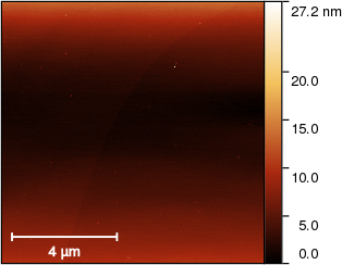
Sample data 1: Monoatomic silicon step
Description: Measurement on monoatomic silicon steps, with considerable interference effects, scanner bow and various local defects. The reported value should be the step height, determined by any Gwyddion function you consider suitable.
Note that the scanner was not calibrated (intentionally), so the correct value is not necessarily the silicon lattice spacing.
Reported value: Step height (single value, in nanometres).
Result
The submitted values are displayed in the following random beehive plot (i.e. vertical positions of the dots help visualising the point density, they do not represent any quantity). Note that a few order-of-magnitude wrong outliers were excluded and attributed to misunderstanding, wrong units, etc.
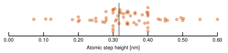
In this case we do not know the correct value precisely. We had essentially two ways of obtaining a ‘correct’ value.
Either by assuming that the step height is exactly what the literature says and using the instrument calibration (known to us) to calculate the step height that should be read from the image. Or measuring the step ourselves from the image as well as we can.
The first method gives 0.317 nm. It is denoted by the grey bar in the graph.
The second method gives 0.32 nm.
The relative error can be up to 10 % in this case.
Estimation
First a few remarks on the theoretical estimation of what value we should obtain from the image.
The silicon step sample, manufactured by Physikalisch Technische Bundesanstalt, Germany, was measured Icon microscope (Bruker). A default calibration of the instrument was used only, which leads to correction factor of 0.984 in the z-axis with the uncertainty of 1.2 %. If a lower uncertainty would be needed, a comparative measurement with a step height standard would be performed, or interferometer based device would be used which was not done in this case.
A reference value for the step height 0.312 ± 0.012 nm can be found in Dixon et al., Silicon single atom steps as AFM height standards, Proc. SPIE 4344, Metrology, Inspection, and Process Control for Microlithography XV, 157 (2001). By dividing it with the correction factor (i.e. performing the opposite of correcting the data) we arrive at the value 0.317 nm listed above.
Oldschool evaluation
The classic evaluation consists in taking profiles. So this was also done for reference.
First

was used to recalibrate the data by multipkying them by the factor of 0.984. Note this is something you could not do (nor was expected to). So the result of this method needs to be compared to the reference step height.
Then Mask of Outliers and Remove Data Under Mask were used to remove the few bright spots on the sample and the mask was removed.
For row levelling

was used with the Median method.
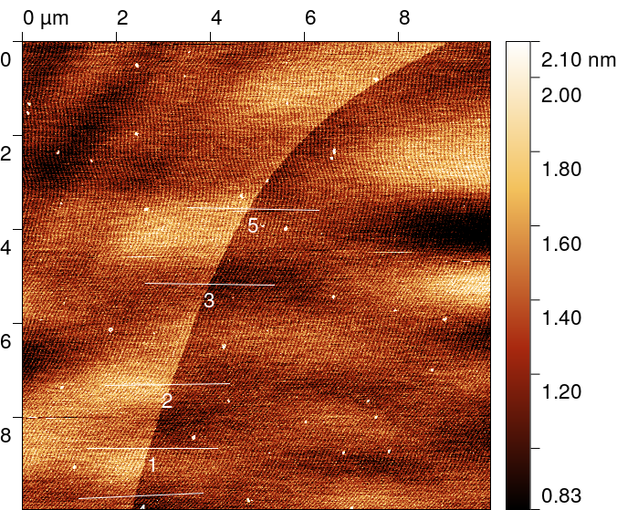
Five profiles of length 2.5 µm and thickness of 20 px were taken using

across the step, preferably in the fast scanning axis direction, trying to avoid too much distortion by the image background.
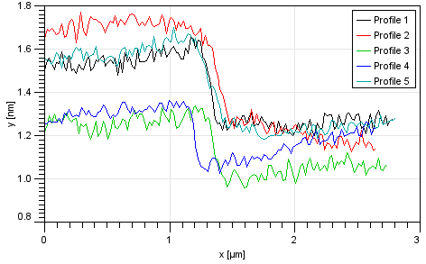
The graph function

was used to fit the step on every profile.
The resulting average value of all the profiles was 0.31. Uncertainty, obtained from fitting error and from average of the profiles was 0.09.
If the recalibration of the data had not been performed during the procedure (as you could not do this step not knowing the coefficient), the resulting value would have been only slightly different: 0.32 ± 0.09.
Note that if a full uncertainty budget would be calculated, it would contain also some other systematic errors of the instrument and uncertainty of this particular measurement would be bigger.
Elegant evaluation
The task is certainly challenging, essentially it is a more difficult variant of the smooth artificial step image. Even though the step is much sharper, there are more artifiacts such as the high-frequency hum and slowly changing background, and the edge is curved. We would like to use the same approach, i.e. calculating column averages or medians and fit them. However, this requires the edge to be vertical.
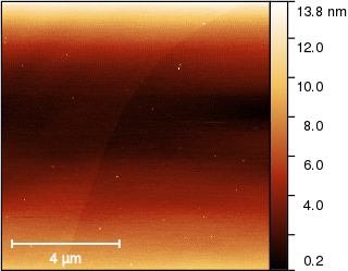
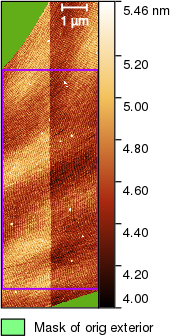
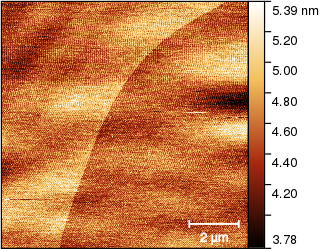
First we need to see the edge. The default colour mapping makes it diffucult to see so we use

and set it to Automatic colour range with tail cut off which prevents the dots on the surface from influencing the mapping:
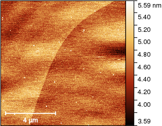
The next step is correction of row misalignment (or bow in the slow axis). The standard function is
and for a rough alignment several of the available methods are equally good. Using Median we obtain
Now we can finally extract the edge and make it vertical. And there is a function for that:
If you start complaining now that there was no such function in Gwyddion when you participated in the survey you are absolutely right. In fact, the function first appears in version 2.45 which has not even been released yet at the time of writing this. So consider this an advertisement. An alternative method that we used originally is described below.
We choose a suitable path along the edge:
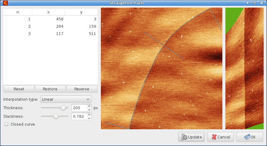
and obtain the following image
Calculating column medians from the selected rectangle produces the following graph
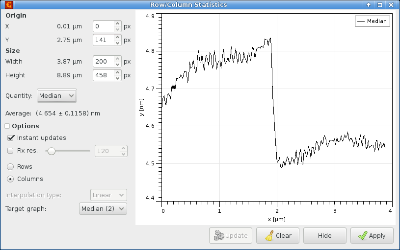
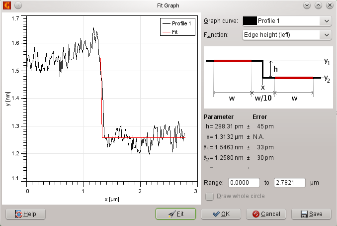
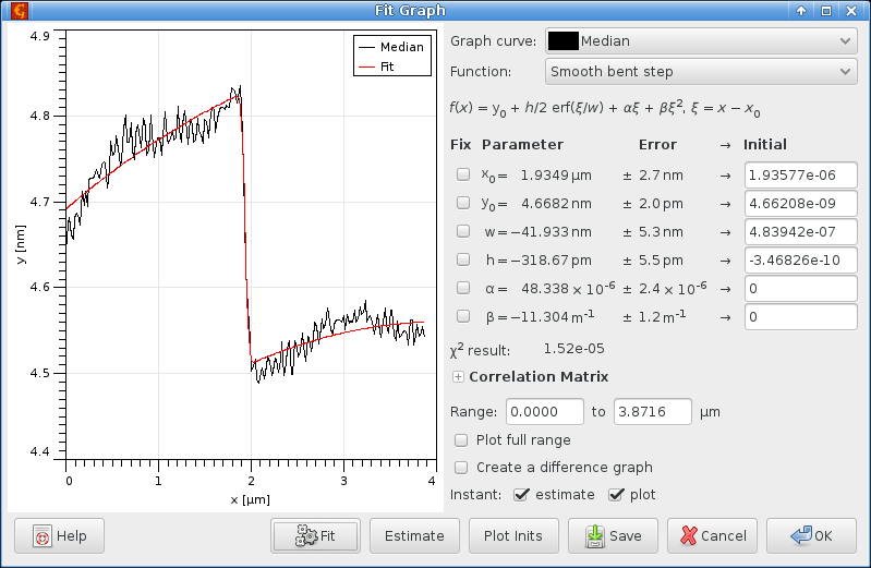
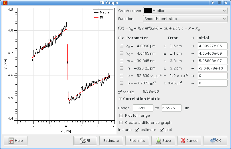
which we fit using

choosing the Smooth bent step function, and obtain the following results:
Exclusive evaluation
Beside questions as whether the plateau around the step are sufficiently wide for correct step evaluation (which participants in the survey had no means to influence), the procedure in the preceding section has two other problems:
- The Straighten Path function was not available in any stable Gwyddion version.
- The function distorts the image in plane, mixing data from different scan rows. It would be nice to exclude any such operations and keep individual scan rows intact.
Hence after row alignment we deviate from the above procedure. First we get rid of the dots on the surface. This can be done using:
with suitable settings
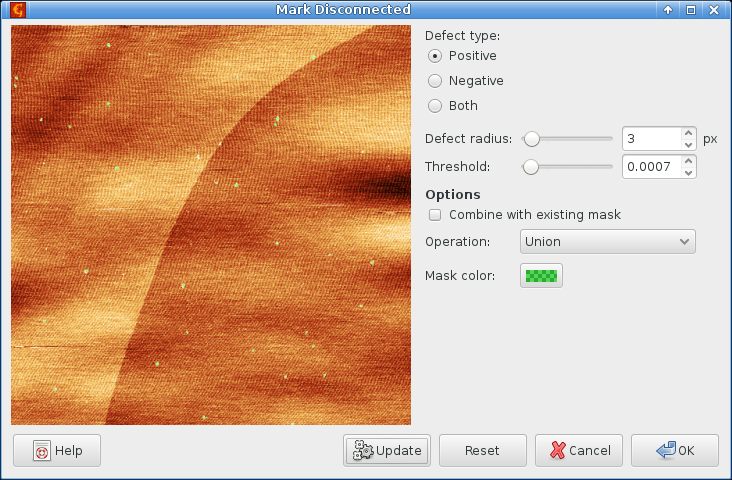
Then we use the the

and Grow the mask by a couple of pixels, ensuring the dots are well covered. Finally we interpolate the masked areas using

and remove the mask, obtaining
Now we have to mark the edge somehow. One option is using one of the edge detection functions but the high-frequency noise makes it difficult. The noise can be suppressed using 1D FFT Filtering, a denoising filter Gaussian filter in the Filters tool or other means. But that starts to sound complicated. Instead, we just use the mask editor tool again and draw a line along the edge:
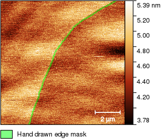
The mask does not have to be very precise because the step evaluation method copes well with wobbly edges. Now we extract the mask to a new data channel using
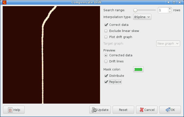
and apply

to the extracted mask image. This is a trick.
Selecting search range of a single row makes the function follow the line closely. Of course, correcting the mask image is pointless, we need to correct the original data. This can be done by enabling the option Distribute which applies the same correction to all compatible channels.
The drift correction only shifts data in individual rows to the left and right. It never mixes data from different rows, which is why we chose it. It does not work well when the ‘drift’ is extremely large so the first attempt straightens nicely the lower part of the edge but keeps the upper part slanted:
This can be improved somewhat by repeating the correction. However, the step is too close to edge of usable data in the upper part anyway. Therefore we just select a reasonable area around the edge
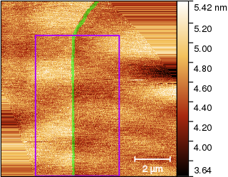
and fit the column medians as before:
We obtained a similar value as before, though not same. Both procedures require significant user input. And although they are relatively robust and when a manual selection is made it can be quite apprioximate, it is possible to obtain values varying between approximately 0.31 and 0.33. This more or less corresponds to the estimated precision with which the step height can be obtained.
